Real-time Machine Learning Detection of Water Pollution using Convolutional Neural Networks
ABSTRACT
India faces a severe water pollution crisis, impacting public health and ecosystems. This project proposes a machine learning model using Convolutional Neural Networks (CNNs) and Multi-Layer Perceptrons (MLPs) that analyze real-time data to create an early warning system for increased pollution rates. This system can empower communities, authorities, and the public to take proactive measures, raising awareness and promoting water resource protection. The project builds upon existing research and datasets, using various forms of data augmentation and two different machine-learning models for detecting the mode of pollution. The CNN model outperformed the MLP model due to its ability to understand spatial relations, leading it to have a 195.6% decrease in loss compared to the MLP model. We introduce a model capable of real-time inference in under 20 milliseconds, leveraging TinyML techniques to quantize our architecture, resulting in a 90% reduction in model size.
INTRODUCTION.
India is grappling with a staggering level of water pollution, which has a severe impact on public health, with an estimated 500,000 deaths [1] annually attributed to waterborne diseases. Moreover, various ecosystems are under significant stress, with nearly 80% of rivers and lakes facing serious degradation due to pollution. The increase in water pollution has been relentless, with a 55% rise in pollution levels over the last decade alone in India.
In response to these statistics, the implementation of devices containing machine learning models offers hope for mitigating the impact of water pollution on the people of India. This system can be used by communities such as farmers near rivers to aid them in preventing crop damage due to high levels of water pollution. Such a system will help prevent losses due to crop failure and prevent the spread of waterborne diseases. By analyzing real-time data, the model can function as an early warning system by detecting when there is an increase in pollutants flowing in water bodies, helping to prevent potential hazards caused by large plastic accumulations. This timely intervention will play a crucial role in safeguarding public health and protecting vulnerable ecosystems. By leveraging data-driven insights, this machine learning model has the potential to make a significant difference in combating water pollution and promoting a sustainable and healthy environment for the people of India.
Implementing devices that can trigger an early warning system can empower local communities and authorities to take proactive measures. By alerting them to potential pollution events and their locations, authorities can mobilize resources more efficiently and implement preventive measures, reducing the impact of water contamination on their lives. An early warning system can also play a vital role in raising public awareness about water pollution. By sharing alerts and information with the general public, the model can foster a sense of responsibility and encourage individual actions to protect water resources.
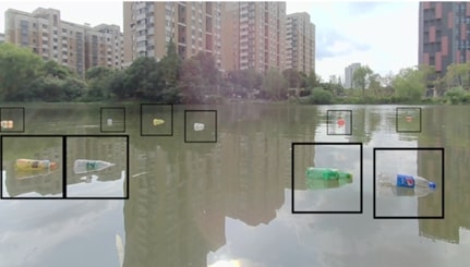
In this study, we introduce a machine learning model specifically trained to detect contaminants present on water surfaces using convolutional neural networks. By generating bounding boxes, the model locates these pollutants. Our model can recognize floating objects in just 20 milliseconds, underscoring its real-time efficacy in monitoring waterways. Our model’s output, as seen in Figure 1, can be used to identify the number of pollutants, and once a threshold is exceeded, an early warning can be sent out to help with mitigation. This CNN model is also compared to a Multi-Layer Perceptron model.
MATERIALS AND METHODS.
The training and testing dataset comprises a total of 2,000, 1280 x 720 images, each annotated with a corresponding XML file, which is a text-based document that stores data in the form of hierarchical elements. XML files are used to store, transmit, and reconstruct data. For the training set these XML files provide information regarding the number of pollutants present in each image, including their location through bounding boxes in the form of (x, y) coordinates. These pollutants mainly include plastic products. The dataset was sourced from previous research [3].
In our image localization project, we are utilizing a CNN, which was trained using this dataset due to its effectiveness in handling variations in images. Our approach involves passing the three RGB color channels as inputs to the CNN. Our CNN model follows a typical architecture, where each component serves a fundamental purpose: the convolutional layer is responsible for extracting features from the input images using filters, the pooling layer aims to reduce dimensionality to enhance computational efficiency while preserving critical features, the dropout layer is utilized to mitigate overfitting by randomly disabling some of the units during the training process, and the flatten layer transforms the multi-dimensional output into a one-dimensional array.
To compare the effectiveness of different neural network models we compared this CNN to a MLP model. The model takes input images with dimensions of image height, image width, and the number of color channels, and flattens them into a 1D vector. It then consists of a sequence of dense (fully connected) layers with rectified linear unit (ReLU) activation functions with a varying number of nodes in each dense layer. Dense layers are fundamental components of a neural network that process the input by performing weighted sums followed by the activation function, essentially enabling the network to learn complex patterns from the data. The final layer employs a linear activation function and generates an output that corresponds to the dimensions required for predicting the coordinates of multiple bounding boxes, specifically, the number of bounding boxes to predict multiplied by 4. This output allows for object detection where identifying the precise location of objects is required. The architecture allows for customization by varying the number of nodes in the dense layers, an adjustment that can be made based on specific requirements.
The objective of our neural network is to predict the position of objects within the image. We detect each object using a bounding box (x1, y1), (x2, y2), that describes the corners of the box that bound the image. To enable our model to detect multiple objects, we will multiply the bounding box dimensions (x1, y1, x2, y2) by the number of objects we want to detect to get the number of output nodes of our fully connected neural network portion of our CNN model. This approach enables our model to identify multiple objects simultaneously within a single inference cycle of our image recognition system.
To get some information about what our image dataset contains, we gathered the summary statistics of objects found within the images. The average number of objects per image is 2.53 with the minimum being 1 and the maximum being 17. Furthermore, we visualize the distribution of the number of objects found within the dataset in a histogram. The histogram indicates that most of our images have only a couple of objects. The distribution is skewed right and indicates that most of our images will only have 1 to 3 objects most frequently.
We are also interested in discerning the prevalent locations of objects within the images. Understanding the distribution of objects within images is crucial as it enhances the generalizability of a model. This knowledge aids in building a more robust predictive model that can accurately detect pollutants across various scenarios. To achieve this, we extracted the bounding box information from the images and employed this data to generate a heat map. This heat map serves as a visual representation of the frequently occurring object locations within the images.
Figure 2, shows a clear trend: the majority of objects detected are in the central region of the images. The majority of the detected objects are concentrated towards the central region of the images. Conversely, there appears to be a notable absence of objects near the upper portion of the images. This observation holds significant implications. It suggests that a model trained on these data will struggle to learn the characteristics of objects positioned near the top of the images. Consequently, this prompts us to consider strategies for enhancing the model’s capacity to accurately predict pollutants situated in recurring positions.

Given that a significant portion of our dataset originates from a single location, we found that a substantial similarity might exist among the images within our collection. This raises the concern that a model trained on such homogeneous data might exhibit limited adaptability when faced with more diverse data sources or varying environments. To gauge the extent of image similarity quantitatively, we leverage the `sklearn` similarity index package. This tool allows us to compute a similarity index, showing the degree of likeness between images.
The outcomes of our analysis reveal a notable pattern. The majority of images share a similarity index that hovers within the range of 0.3 to 0.5. This range serves as an indicator that our dataset indeed comprises images with substantial similarities. Acknowledging this outcome reinforces the need for careful consideration when training our model, as its performance might be disproportionately influenced by the concentrated similarity within our data. To combat this, we used various data augmentation techniques to our data which included image rotation, zooming, and scaling. By applying these transformations to the existing training data, we generated new examples that are variations of the original ones. This helped generalize the model.
RESULTS.
The performance comparison between CNN and MLP yielded compelling results. The numerical outcomes demonstrate a significant disparity in the model performances, as evidenced by the stark contrast in their respective loss values. The validation loss is a numerical value that indicates how well the model performs on the validation dataset. It is calculated using a loss function that measures the discrepancy between the model’s predictions and the actual target values in the validation set. The loss function used was mean squared error (MSE) which is a commonly used metric in machine learning and regression tasks, including neural network training. It measures the average squared difference between the predicted values and the actual values in a dataset. Here, MSE quantifies the average squared difference between the predicted positions of pollutants by the models (MLP and CNN) and their actual positions in the validation dataset.
After training both models for 20 epochs the CNN model reported a 195.6% decrease in the loss compared to the MLP model. Where epochs refer to a single cycle of training the neural network with all the training data. These findings indicate a notable advantage of the CNN architecture in effectively addressing the complexities inherent in the real-time monitoring data associated with water pollution events.
DISCUSSION.
Our investigation initially focused on comparing MLPs and CNNs in the context of our image recognition project. The comparative analysis provided valuable insights into the performance of these machine learning architectures. While MLPs offer flexibility in their architecture, CNNs, which operate at the feature level, tend to be better suited for image data due to their ability to capture spatial relationships.
To gain a deeper understanding, we conducted experiments with various MLP architectures. We observed that MLP architectures with greater height and width tended to exhibit superior performance, which, in this context, means achieving a lower loss score indicating a closer match between the model’s predictions and the actual data. This phenomenon can be attributed to the increased complexity of functions within these architectures. Even with varying the different MLP architectures, their predictions were still not good enough to identify plastic accurately.
One significant limitation lies in the flattening process, which results in the loss of spatial information between pixels in the image. This is crucial in image processing and object localization processes since a cluster of pixels that represent plastic are usually clustered in the x and y dimensions. The flattening process leads to the loss of this information, which is very important to the identification of the plastic.
This drawback led us to explore CNNs further. CNNs offer distinct advantages, as they operate at the feature level instead of the pixel level. This characteristic makes them particularly well-suited for image data, as they keep the spatial structure of the image intact.
Our testing with CNN provided for a much lower error rate compared to our MLP model, as shown in Figure 3. For the MLP Model it begins at a validation loss of 13,877,020,672.0000, whereas for the CNN model, it begins at a validation loss of 155,520.4219. This is because CNNs are designed to account for spatial hierarchies in data, making them well-suited for tasks like image processing and object detection. They can automatically learn hierarchical features through convolution layers. Such hierarchical features include edges, textures, and shapes, which are crucial for identifying objects in images.

CNNs employ convolutional layers that apply filters to extract local patterns and features from images. These filters capture various aspects of the data, and their shared weights allow the model to recognize these patterns regardless of their location in the image. Moreover, we used 4 convolutional layers with a filter size of 32, which represents the dimensions of the convolutional kernels used in each layer. This filter size determines the receptive field of the convolution operation, influencing the feature extraction process within our CNN. The filter size of 32 yielded the most accurate and credible results. However, to address the common challenge of overfitting in deep learning, we also implemented dropout layers in our model. These dropout layers played a crucial role in regularizing the network by preventing it from becoming too reliant on specific features or patterns in the training data. The drop-out layers aim to take a first step towards tackling the high similarity of our dataset and the concentration of pollutants towards the center of our image.
Lastly, our CNN included pooling layers that reduce the spatial dimensions of the feature maps while retaining valuable information. This helps to create a representation of the image’s content, which is vital for object detection tasks.
Furthermore, the practical deployment of machine learning models for real-time monitoring in remote locations, such as rivers in the context of our project, presents a unique set of challenges. Large-scale models that perform exceptionally well on high-performance computing systems can be impractical for deployment on resource-constrained embedded devices, which are often powered by limited energy sources. To address this challenge, our research emphasizes the utilization of smaller machine-learning models tailored for embedded devices.
TensorFlow’s quantization was used to make this model more efficient for deployment on devices with limited resources, like the ones which will be deployed along the water sources. During the initial training of a neural network, high-precision values, such as 32-bit floating-point numbers, are commonly used to ensure accuracy. After training, the quantization process is applied, which involves reducing the precision of the model’s weights and activations to lower bit-width representations, such as 8-bit integers. This reduction in precision helps save memory and accelerates inference on hardware with limited computational capabilities. As a result, we were able to achieve a remarkable size reduction of 91% of the original model size.
CONCLUSION.
In conclusion, the research undertaken to investigate the utilization of machine learning techniques for early warning systems in water pollution events has yielded valuable insights. Among the models tested, CNN has emerged as the most effective in leveraging real-time monitoring data for this critical task. Its superior performance in handling spatial features within the data, such as identifying pollutants in images or time-series data, has demonstrated its ability to provide timely alerts for potential water pollution events.
Looking ahead we plan to explore various data augmentation techniques to increase the generalizability of our model. We also plan to improve this model by increasing the types of pollutants it can detect, for example: oil spills, plastics, harmful algae, and sewage.
Furthermore, the study’s generality can be enhanced by diversifying the types of machine learning techniques employed. In future investigations, we intend to incorporate other algorithms, such as Recurrent Neural Networks (RNNs) for time-series data analysis, Random Forests for ensemble learning, or Support Vector Machines (SVMs) for classification tasks.
SUPPORTING INFORMATION.
All the code behind the project can be found at https://github.com/Veer2906/Real-Time-Water-Pollution-Detection.git
ACKNOWLEDGEMENTS
Thank you for the guidance of Jason Jabbour, my mentor from Harvard University in the development of this research paper.
REFERENCES.
- Lancet study: Pollution killed 2.3 million Indians in 2019. EPIC (2022), (available at https://epic.uchicago.edu/news/lancet-study-pollution killed-2-3-million-indians-in-2019/).
- Central Pollution Control Board. CPCB, (available at https://cpcb.nic.in/nwmp-data/).
- Y. Cheng, J. Zhu, FloW: A Dataset and Benchmark for Floating Waste Detection in Inland Waters. (available at https://ieeexplore.ieee.org/document/9710581)
- Alzubaidi, L., Zhang, J., Humaidi, A.J. et al. Review of deep learning: concepts, CNN architectures, challenges, applications, future directions. J Big Data 8, 53 (2021).

Posted by buchanle on Tuesday, April 30, 2024 in May 2024.
Tags: Machine learning, real-time, Water-Pollution