Water Potability Prediction with Machine Learning
ABSTRACT
In today’s world, humanitarian conflict affects the lives of millions. In 2010, the United Nations recognized that access to potable drinking water was a human right [1]. At the time that this established, 884 million people did not have access to potable water, and 2.6 billion people did not have access to basic sanitation [2]. In this paper, we propose a machine learning driven tool to clarify the quality of water using an analysis of the correlations between socioeconomic indicators (mortality, prevalence of diseases, …) and access to fundamental drinking water services. Using these data analyses as context, we build a machine learning tool to predict water potability for a water sample. We train and fit many different machine learning models to find the best algorithm, for which we optimize its parameters to build a final working tool.
INTRODUCTION.
Every day, Earth’s global population rapidly increases, straining the planet’s resources as it accommodates 73 million more individuals annually and their fundamental necessities: food, water, and shelter [3]. According to NASA, Earth is 71 percent water, but less than 3 percent of that water can be used for drinking [4]. As the amount of drinkable water stays constant but the global population increases, it calls to attention the state of current available water supply, and the implications on populations who already do not have access to healthy supplies. In particular, the repercussions from drinking water of inadequate standards affect over 2 billion people around the world according to the World Health Organization [5]. The greatest risk for populations is drinking water contaminated with feces in addition to the possibility of “microbiologically contaminated” water that can “transmit diseases such as cholera, dysentery, typhoid, and polio” [5]. The 17 Goals of the United Nations encompass various aspects of human society, number 6 being “Clean Water and Sanitation”, a goal we aim to address [6]. In the past, others have attempted to address this issue using different datasets. However, the quality of the datasets had a large impact on the accuracy of the models. For this experiment, a different dataset was utilized and a data analysis between various features and their correlation to that region’s basic drinking water services was performed. From these analyses the observed patterns were used as a foundation to build a tool that predicts a water sample’s potability by utilizing training and fitting machine learning models.
MATERIALS AND METHODS.
First Dataset Introduction.
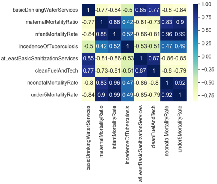
To understand the effect that water potability has on populations and its correlation with various factors (e.g. maternal mortality rate), a dataset that measured these factors in various regions around the world was utilized. This dataset was subsampled from a larger metadataset called “World Health Statistics 2020 | Complete | Geo-Analysis” [7]. The available data about drinking water services and various factors that were believed to be related to drinking water services were combined. The subsampled dataset created holds 2,792 data points over 8 features. The features describe basic drinking water services, maternal mortality, infant mortality, incidence of tuberculosis, basic sanitation services, clean fuel and technology, neonatal mortality, and mortality under the age of five. In Figure 1, we note that there is some significant correlation between features which we will utilize as context for the results of our prediction tool.
Correlations are the measure of the mathematical linear relationship between two variables [8]. A positive correlation occurs when both variables increase or decrease the same way, a direct relationship. This type of correlation is measured from 0 to 1. A negative correlation occurs when the variables increase or decrease in opposite directions, modeling an inverse relationship. This correlation is measured from -1 to 0. If a correlation is close to 0, the two variables are minimally related. Correlation calculations follow this formula where is the correlation coefficient, represents the x-variables, represents the mean of the x-values, represents the y-variables, and is the mean of the y-values [8]:
\[r_{xy} = \frac{(\sum_i x_i-\overline{x})(y_i-\overline{y})} {\sqrt{\sum_i(x_i-\overline{x})^2\sum_i(y_i-\overline{y})^2}}\tag{1}\]
Second Dataset Introduction.
Understanding these correlations gives more context to the water potability prediction tool we aim to build. In the past, others have used similar datasets to find the optimal machine learning model that predicts a water sample’s potability. One such paper tested K-Nearest Neighbors, Logistic Regression, and Random Forest models after following a data cleaning process that we explored as well [9]. The paper found accuracies from 60-70% for all models, which is relatively low, most likely due to the data being synthetic without representative distributions of data. For example, in Figure 2 below, the distribution of the Hardness and Solids features are shown, respectively. It is evident that the distributions of the points are very similar, regardless of whether the water is potable or not. The models are unable to learn because there is no difference between the clean and dirty water data points, hence the low accuracies.
For our prediction tool, a dataset called “Water Quality” was utilized [10]. Holding 7,999 data points with 21 features each, the data encompasses aspects of water quality and determines if those factors make the water potable or not. The factors are as follows: aluminum, ammonia, arsenic, barium, cadmium, chloramine, chromium, copper, fluoride, bacteria, viruses, lead, nitrates, nitrites, mercury, perchlorate, radium, selenium, silver, uranium, and is safe (whether that sample is safe to drink or not). The null values were removed, and the classification task, whether a sample is potable or not, was established. In this dataset, 11.4% of the data is potable, while the other 88.6% is not. This imbalance will be taken care of when computing accuracies later.
Machine Learning: PCA Analysis
The following shows the heatmap of the correlations of the features in the new dataset. Lighter colors correspond to lower correlations, and vice versa. Correlation between some features, such as chloramine and perchlorate was noted, which allows us to perform PCA analysis. For this experiment, the results of this PCA analysis are used strictly for comparison.
In Figure 3, we note that some correlations exist among the features of the dataset, indicated that PCA Analysis can be done. The objective of Principal Component Analysis (PCA) is to take the many interrelated features of a dataset and form new features or reduced dimensions (the principal components) that are all uncorrelated but still maintain the components responsible for most of the variation that the original data had [11]. To perform PCA, the covariance matrix of the dataset is computed. Next, we compute the eigenvectors from that covariance matrix. The eigenvector with the highest eigenvalue represents the direction with the highest variance, producing the first principal component. This pattern continues, using the second highest eigenvalue to reveal the second principal component, and so forth [12]. The formula to calculate the covariance matrices is:
\[cov(x,y) = \frac{1}{n-1}\sum_{i=1}^{n}(x_i-\overline{x})(y_i-\overline{y})\tag{2}\]
Machine Learning: Models.
Various models were utilized in finding different accuracies of predictions. XGB Classifier, Decision Tree Classifier, and Random Forest Classifier yielded the best results.
XGBClassifier: The Extreme Gradient Boosting (XGB) Classifier is a classifier that utilizes the predictions of weaker models to then provide a more accurate output. This system is called ensemble learning [13]. The XGB classifier implements the gradient boosted trees algorithm, which works due to decision trees and gradient boosting [14]. A decision tree is a “tree” with a root and its nodes that organizes data and makes it easier to create a classification model based on the information. XGBoost also includes a “max_depth” parameter that “specifies the stopping criteria for the splitting of the branch, and starts pruning trees backwards” [15]. This process allows the model to significantly improve its accuracy [15]. In addition to tree pruning, XGBoost utilizes regularization to “counter overfitting models by lowering variance while increasing some bias” [16]. XGBoost employs other methods such as parallelization, sparsity awareness, and cross-validation. Gradient boosting is an ensemble method (mentioned previously) [14]. These two techniques come together and allow the XGB classifier to predict with higher accuracies than other models.
DecisionTreeClassifier: The Decision Tree Classifier is an algorithm that works by utilizing decision trees to make its predictions [17]. From the nodes of the decision tree, the algorithm splits the data into subsets based on each node’s most significant feature. This “splitting” of the data needs to be controlled in order to not overfit the model, and this can be adjusted using the parameters of the algorithm [17]. Additionally, the Decision Tree Classifier implements entropy, the uncertainty or error in a node of a decision tree. Since in a decision tree, the output is usually binary, with either a “yes” or “no”, entropy can be found using the following formula, where is the probability of positive cases, is the probability of negative cases, and is the subset of the training set,
\[E(S)=-p_{(+)}logp_{(+)}+p_{(-)}logp_{(-)}\tag{3}\]
After understanding the errors in a node, the algorithm utilizes information gain, which measures the reduction of the error [17]. Information gain builds on the information found from the entropy using the following formula, which in simpler terms is entropy of the entire dataset minus the entropy of a feature of that dataset,
\[Information Gain = E(Y) – E(Y|X)\tag{4}\]
RandomForestClassifier: The Random Forest Classifier is an algorithm that utilizes bagging and boosting, techniques mentioned before, that are present in the XGB Classifier algorithm. This classifier heavily relies on decision trees. Bagging, or Bootstrap Aggregation, works by taking random subsets of the original data and training them individually to generate outcomes [18]. This step is called row sampling, or bootstrap. Once all the individual models are trained, their results are combined, and based on majority voting, form a final result. This step is called aggregation [18]. Boosting is another technique that the Random Forest classifier utilizes. Like other ensemble learning methods, boosting algorithms combine simpler models to get a more accurate result [18]. Putting the two together, first, random samples and features are chosen from a dataset and decision trees are made for each sample. Next, each decision tree provides an output. Those outputs are then combined and, based on majority voting, a final result is obtained [15].
RESULTS.
PCA Analysis.
Because some features are correlated, it indicates that dimensionality of the dataset can be reduced using PCA upon analyzing the variance that the different components account for (Fig. S2). We see from the cumulative sum of the eigenvalues (Fig. S3) that around 12 components are needed to capture 95% of the variance (the x-value where the red and blue line intersect).
Model Accuracies.
After preprocessing the dataset and determining the classification task, we split the data into the training and testing sets. The data was then scaled and a grid search was used to determine the optimal parameters for each model that was being tested. After the best parameters were inputted into each model, the Decision Tree Classifier gave an accuracy of 96.44%, XGB had an accuracy of 96.38%, and Random Forest had an accuracy of 95.88%. Figures S4-S6 depict the confusion matrices for the three models, respectively. To take into account the large imbalance of potable and not potable points, weighted averages of all three models were found as well. Weighted averages or balanced accuracy is equal to the average of the true positive rate (sensitivity) and true negative rate (specificity) [19]. The formula used to calculate these balanced accuracies is as follows,
\[\frac{1}{2} \left(\frac{TP}{TP+FN}+\frac{TN}{TN+FP}\right)\tag{5}\]
where TP = true positives, TN = true negatives, FP = false positives, and FN = false negatives.
DISCUSSION.
Correlation Analysis.
Figure S1 illustrates a visual representation of the pairwise correlations between the features in this dataset (Fig. S1). Upon analysis, it is observed that the feature that has the highest positive correlation with basic drinking water services is basic sanitation services with a correlation coefficient of 0.85. Water, sanitation, and hygiene services (WASH) are facilities that significantly increase standards of life in both urban and rural regions. In an analysis of WASH facility data of 14,156 households, a correlation between basic drinking water and sanitation services is seen [20]. From the households, 64% had access to basic drinking services, but only 13.28% had access to basic sanitation services. However, the same factors affected both water and sanitation positively: female-headed households, wealthy households, and household-heads older than thirty. Being impacted by the same factors could explain the correlation between the two features.
The two most negatively correlated features with basic drinking water services are infant mortality rate and under 5 mortality, both with a correlation coefficient of -0.84. According to the World Health Organization, no access to WASH facilities results in 2 million deaths worldwide, most of them being children [20]. One of the main causes of these deaths are due to the inadequate water supply, which creates an environment in which disease rapidly spreads. For example, diarrhea, one of these rapidly transmitted diseases, sees 1.7 billion cases in children under 5 years of age with 446,000 succumbing to the disease each year [21]. According to the CDC, universal access to the WASH facilities can reduce global disease by 10%, explaining the negative correlation between the features, that increased basic drinking services are correlated with decreasing infant and under 5 mortality rates.
PCA Analysis.
Through the PCA Analysis, the dimensions of the dataset were reduced, and it was determined that 12 components can be used to capture 95% of the variance. Although we did not utilize PCA analysis for training models in this experiment, the results can be utilized for machine learning in future projects.
Accuracies.
From the model summary (Table S1), we can see that the Decision Tree Classifier was determined to have the highest accuracy of 96.44%. Although the accuracy could be higher, this water potability prediction tool can be used to elucidate the quality of water in water-stressed regions. The utilization of grid search helped to tune the parameters (Table S2) and increase the previous accuracies. The confusion matrices (Fig. S4, Fig. S5, Fig. S6) depict where the model predicted wrong. When it comes to errors in all of the confusion matrices, there is an inherent bias towards type II errors, or false negatives. Ensuring this bias towards type II errors is important for prioritizing the accurate prediction of water potability, recognizing that it is safer to overestimate water contamination rather than the potential negative impact of being unable to distinguish harmful conditions. Compared to the paper previously mentioned, the false positives found in this experiment are less than those produced from the paper’s RF, ANN, and K-NN algorithms [9]. However, the paper’s LR algorithm predicted 0 false positives. Although the LR algorithm’s accuracy is not as high as the algorithms utilized in this experiment, it’s type I error rate is much more efficient. To improve our false positive rates, we could use other methods and models that optimize the results efficiently. One such method could be using cross-validation, a method that allows for the training and validation of models by rotating the use of different data segments [22].
Compared to the research mentioned before with accuracies of 60-70%, this dataset had much better results [9]. Although we used similar models, the difference in results shows that this synthesized dataset had more distribution than the one used in the referenced paper. However, the work with the models still gives context on water potability, an issue that is still prominent in many rural regions.
CONCLUSION.
As machine learning continues to improve, it is essential to take advantage of its abilities. The UN has stated that at least 3 billion people live not knowing the state of their water quality due to a lack of monitoring and resources [6]. In this paper, factors that affected basic drinking services were analyzed, and used those observations as context to build a water potability prediction tool. Training and fitting models, we found results with accuracies of 95% and higher. Once building this prediction tool, we hope individuals can utilize it to provide a basic understanding of the water quality in the regions they live in. It is important not to engage in over-reliance on this tool, but to use it with other resources to confirm its predictions. For future projects, it may be illuminating for researchers to consider what factors in an area may lead to type II errors and use that understanding to strengthen the model’s accuracy, minimizing those false positives.
ACKNOWLEDGMENTS.
The work was supported by the Veritas AI program. The authors would like to thank Constance Ferragu at Princeton University for her guidance in machine learning and data science.
SUPPORTING INFORMATION.
Additional supporting information includes:
Figure S1. Visual representation of correlations
Figure S2. Variance Graph
Figure S3. Cumulative Graph
Figure S4. Decision Tree Classifier Confusion Matrix
Figure S5. XGB Confusion Matrix
Figure S6. Random Forest Confusion Matrix
Table S1. Summary of Model Summaries
Table S2. Optimal Parameters
REFERENCES.
1 Human right to water and sanitation. United Nations Department of Economic and Social Affairs. https://www.un.org/waterforlifedecade/human_right_to_water.shtml#:~:text=In%20November%202002%2C%20the%20Committee,a%20life%20in%20human%20dignity. (accessed Feb. 25, 2024).
2 General Assembly declares access to clean water and sanitation is a human right. United Nations (2010). https://news.un.org/en/story/2010/07/346122 (accessed Feb. 25, 2024).
3 World Population Clock. https://www.worldometers.info/world-population/#:~:text=Population%20in%20the%20world%20is,it%20was%20at%20around%202%25 (accessed Feb. 25, 2024).
4 J. Nemeth-Harn, How much water on Earth is drinkable?. Hard R/O Systems Blog (2020). https://blog.harnrosystems.com/how-much-water-on-earth-is-drinkable (accessed Jul. 27, 2023).
5 Drinking-water. World Health Organization (2023). https://www.who. int/news-room/fact-sheets/detail/drinking-water (accessed Jul. 27, 2023).
6 Make the SDGs a reality. United Nations Department of Economic and Social Affairs. https://sdgs.un.org/goals/goal6 (accessed Jul. 27, 2023).
7 World Health Organization, World Health Statistics 2020|Complete|Geo-Analysis. (2020); https://www.kaggle.com/datasets/utkarshxy/who-worldhealth-statistics-2020-complete (accessed Jul. 27, 2023).
8 Correlation, University of Illinois Urbana-Champaign. https://discovery.cs.illinois.edu/learn/Towards-Machine-Learning/Correlation/ (accessed Jul. 27 2023).
9 D. Poudel, D. Shrestha, S. Bhattarai, A. Ghimire, Comparison of machine learning algorithms in statistically imputed water potability dataset. Journal of Innovations in Engineering Education 5, 38-46 (2022).
10 “Water quality.” (2021); https://www.kaggle.com/datasets/mssmartypants/water-quality. (accessed Jul. 27, 2023).
11 Principal Components Analysis, Carnegie Mellon University. https://www.stat.cmu.edu/~cshalizi/uADA/12/lectures/ch18.pdf (accessed Jul. 27, 2023).
12 Mean Vector and Covariance Matrix, National Institute of Standards and Technology. https://www.itl.nist.gov/div898/handbook/pmc/section5/pmc541.htm (accessed Jul. 27, 2023).
13 Y. Zhang, J. Liu, W. Shen, A Review of Ensemble Learning Algorithms Used in Remote Sensing Applications. Applied Sciences 12, 1-19 (2022).
14 I. Hanif, Implementing Extreme Gradient Boosting (XGBoost) Classifier to Improve Customer Churn Prediction (European Alliance for Innovation, 2019).
15 XGBoost Parameters. https://xgboost.readthedocs.io/en/release_0.90/parameter.html (accessed Apr. 2, 2024).
16 A. Um, L1 L2 Regularization in XGBoost Regression. Medium (2021). https://albertum.medium.com/l1-l2-regularization-in-xgboost-regression-7b2db08a59e0 (accessed Feb. 25, 2024).
17 Y. Song, Y. Lu, Decision tree methods: applications for classification and prediction. Shanghai Arch Psychiatry 27, 130-135 (2015)
18 S. J. Rigatti, Random Forest. Journal of Insurance Medicine 47, 31-39 (2017).
19 Balanced Accuracy Score. Scikit Learn. https://scikit-learn.org/stable/modules/model_evaluation.html#balanced-accuracy-score (accessed Jul. 27, 2023).
20 N. Gaffan, A. Kpozèhouen, C. Dégbey, Y. G. Ahanhanzo, R. G. Kakaï, R. Salamon, Household access to basic drinking water, sanitation and hygiene facilities: secondary analysis of data from the demographic and health survey V, 2017–2018. BMC Public Health 22, (2022).
21 Assessing Access to Water & Sanitation. CDC (2022). https://www.cdc.gov/healthywater/global/assessing.html (accessed Jul. 27, 2023).
22 P. Refaeilzadeh, L. Tang, H. Liu, Cross-Validation. Encyclopedia of Data Base Systems, 532-538 (2009).

Posted by buchanle on Tuesday, April 30, 2024 in May 2024.
Tags: Machine learning, Tool, Water Quality