Utilizing Predictive Models to Detect Parkinson’s Disease Via Fractal Scaling
ABSTRACT
Degenerative diseases can cause many symptoms, most of which have not been explored as a tool for diagnosing. A niche, but prevalent variation in characteristics of those with Parkinson’s Disease includes the voice. The article by Little et al. delves into voice variation, which contains many arbitrary parameters and complex techniques to differentiate. However, fractal scaling emerges as a new technique to simplify the classification using a “hoarseness” diagram to determine normality or disorder from speech, which can distinguish PDpos subjects from PDneg subjects. This method has better classification performance and is utilized in the dataset “Parkinson’s Disease Detection”, maintained by UCI’s Machine Learning Repository. Using various forms of predictive models such as logistic regression, decision trees, and neural networks, this project focuses on using observed parameters from fractal scaling between a PDpos and PDneg voice to aid in the diagnosis of Parkinson’s Disease.
INTRODUCTION.
Neurodegenerative diseases affect millions of people worldwide and are common and complex, with minimal abstract data available regarding them. Within the last decade, innovations have aided in the quick diagnosis of neurodegenerative diseases. However, modern day healthcare has still been unable to perfect a method to effectively diagnose such disorders. This is particularly alarming because quick diagnosis can be pivotal in prognosis, prevention, and subsequent treatment. While in the past decade, factors like family life, genetics, and age have been used, their predictive power is both inconsistent and largely unreliable across patients, making it difficult for accurate and early diagnosis to be possible. Moreover, other diagnostic tools, such as Computed Tomography scans or Magnetic Resonance Imaging, are highly expensive neuroimaging tools and can also be invasive to the patient. Fractal scaling, a method to analyze speech patterns, could be used as a cost-efficient and noninvasive procedure to accurately diagnose Parkinson’s Disease.
Parkinson’s Disease, affecting up to one million in the US alone [1], is a brain disorder caused by a loss of nerve cells and subsequent degeneration within the brain in the Substantia Nigra, which is responsible for producing dopamine. Consequently, Parkinson’s Disease, or PD, greatly affects motor control and movement, causing uncontrollable movements that worsen over time. Currently, diagnosing PD involves reviewing symptoms, medical history, and performing various examinations. There is no specific test to diagnose PD. However, many symptoms that PD typically invokes can be utilized to aid in diagnosis, specifically that of voice. Speech and voice are highly affected by Parkinson’s disease, and 89% of patients experience speech and voice disorders because of Parkinson’s [2].Particularly, it affects vocal and fundamental frequencies within their voice. Previously, predictive models have relied on fundamental frequencies to determine whether someone has a disorder, but instead, using vocal frequencies provided by components of fractal scaling could possibly produce more robust, accurate models. Using a fractal scaling method, a person’s voice can be utilized to diagnose whether they are PDneg, or PDpos. Thus, a predictive model that uses Fractal Scaling properties would help to predict the possibility of PD.
MATERIALS AND METHODS.
Dataset Description and Data Cleaning. The dataset used for this project includes observations from 31 people, 23 with Parkinson’s Disease, and 6 voice samples from each person. The dataset is entitled ‘Parkinson’s Disease Detection’ and was maintained at the ICU Machine Learning Repository [3]. The data considered here was gathered by Little et al. and includes voice metrics analyzed through the aforementioned fractal scaling methods [4]. The attributes it includes are subject name and recording number, average, maximum, and minimum fundamental frequencies, measures of variation in fundamental frequency, tonal components in the voice, various fractal scaling components, and the final health status of the patient. This dataset was then processed, analyzed, and modeled for machine learning, using Python libraries Pandas [5], NumPy [6], Sci-Kit [7], and TensorFlow [8]. After this, a dataset analysis [9] was completed to retrieve summary statistics of the dataset. This was critical to research what key factors of fractal scaling would be most indicative of patient diagnosis. Within this, voices that are deemed PDpos are given a binary value of ‘1.0’, while PDneg is given ‘0.0’. After modeling, a confusion matrix was used as a tool, which is a classification table that represents various outcomes and evaluates the accuracy of a classification.
Exploratory Dataset Analysis. To analyze signal fractal scaling components; a boxplot shows the median and range for signal fractal scaling components. It looks as if the median for fractal scaling components is roughly 72.5%, whereas the range stretches from above 80% to below 60% This implies that while the range is large, there are a greater number of fractal scaling components above 72.5% in this dataset.
Next, the relationship between two attributes: ‘HNR’ and ‘NHR’. These are two measures of noise to tonal voice components in the voice. The graph indicates that they are inversely correlated. As one of them increases, the other one decreases. This relationship between the two measures may be able to indicate whether someone is PDpos or PDneg. For example, if someone has a greater HNR, it would be implied that they have a lower NHR, and that could be PDneg or PDpos.
Exploring NHR and Status; a scatterplot shows NHR on the x axis and status on the y axis. It shows that having an PDpos status is typically only associated with having a lower NHR, however, the data is very erratic and does not have a trend.
Inversely, exploring the relationship between HNR and Status is similarly very erratic. However, it shows that the HNR on the x axis is typically only associated with an PDpos status when the value is higher. However, no clear trend can be derived from this graph.
Finally, analyzing the different distribution of values for every single attribute in the dataset. While some of them have clear trends, some of them do not.
RESULTS AND MODELING.
Logistic Regression. The first model we used was logistic regression. Logistic regression is used for statistical analysis and analyzes relationships and patterns within a dataset to predict a binary outcome. For this dataset, the input variables are the various tonal frequencies and static frequencies of voice, and the output variable is has Parkinson’s, which is a strong indicator of Parkinson’s Disease (1 or 0). Using logistic regression had its respective advantages and disadvantages. The advantages include that the result is easy to interpret, seeing as it is split into a simple binary outcome. Moreover, it is easy to train, particularly with simpler datasets. However, the dataset used had many predictive variables, which led to a drawback with using Logistic Regression. It tends to overfit using high dimensional datasets, which meant permutation tests, such as cross validation, had to be used to assess over fitting and verify the high accuracy. After this test, in implementation, the data was split into a train set of 85% and a test set of 15%; the train set trained the logistic regression model, and then tested the trained model on the test set of data. Figure 1 indicates the varying false negatives and false positives, yielding an accuracy of 87%.
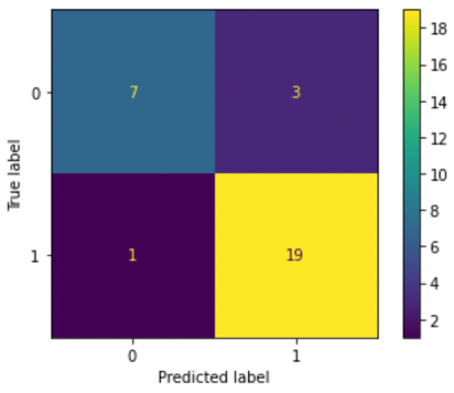
Figure 1. Confusion matrix for logistic regression model. This shows that there are 3 out of 7 false negatives, and 1 out of 19 false positives; all other predictions were right.
Decision Trees. Random forest was the second classification algorithm used to predict accuracy. Again, there is a train set used to train the model; it learns a curve dependent on if else decision rules from the dataset by using various ‘decision trees.’ This model was advantageous in that it was capable in handling multidimensional datasets and can adapt to the various frequencies of voice measured in fractal scaling. Random Forest was created to result in a binary outcome after evaluating all the rules used for other dataset features. However, a drawback is that decision trees, when they become too complex, are bad at generalizing data. This leads to overfitting again. Another drawback is that small outliers in the data might have vastly different results. When finally used in the context of a forest, many of these outcomes based on decision rules can be used to predict a final value, which implies a voice disorder or no voice disorder in this context. For this project, the number of tree nodes was experimented on many times to mitigate running into these problems. We took a series of decision trees and made a random forest. In this model, a test set of 20% was used and a train set of 80% was used. There were many problems with overfitting, where the model fit exactly with the training set. This means that even though the model produced a higher accuracy, it wasn’t necessarily because the model was improving its prediction capabilities. To conclude, we ended up with a model that has 95% accuracy. Figure 2 depicts the accuracy for both positive diagnoses and negative diagnoses.
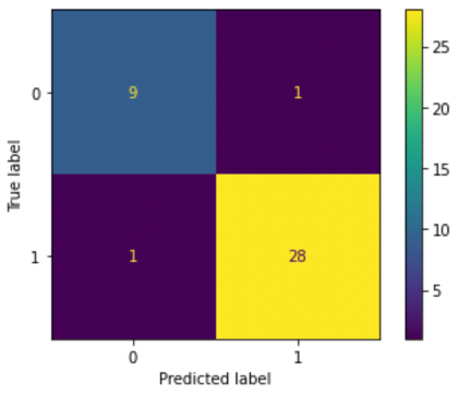
Figure 2. Confusion matrix for random forest model. This shows that there is 1 false negative out of 9, and 1 false positive out of 28; all other predictions were right.
Neural Networks. Neural Networks are the final classification algorithm used: they mimic the human brain by using different nodes to create a network that recognizes the relationship between varying data types. Although these are beneficial because they can handle and store large amounts of data across the entire network, they often can get extremely complicated depending on the number of nodes and networks used. However, they are generally efficient, particularly at multitasking, and are self-improving as they continue data retrieval and constantly increase in accuracy. Again, this was split into a train and test set, where the neural network was trained with data and then used with the test set. The data trained the model using three separate parts; input nodes, weights that the model has learned, and a bias term. These all get summed to create an output node. It mimics human systems of neurons and uses hidden layers to process data until it can find enough patterns to predict an accurate result. For this, we tested different numbers of layers and nodes to build the most accurate model. We used 3 layers and epochs, or number of times the entire dataset passes through the model, of 25, 10, and 2, to result in a best test accuracy of 90%. To train the network, a test set of 15% and a train set was 85% were used. Figure 3 depicts a Confusion Matrix based on the results of the test set. The true label is the true diagnosis of the data row, and the predicted label shows what the Neural Network Model predicted.
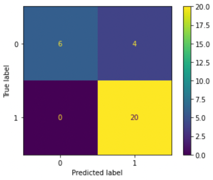
Figure 3. Confusion matrix for neural network model. This shows that there are 0 false negatives out of 6, and 4 false positives out of 20; all other predictions were right.
DISCUSSION.
Now that the data has been collected and cleaned, as depicted in Table 1, and the model has been trained and evaluated by an accuracy measurement, the performance overall can be calculated further to evaluate the effectiveness of the model. The confusion matrix is a method used to evaluate the performance of the model and displays any strengths or shortcomings of the precision. The result is a two-by-two array: predicted outcome by actual outcome. For example, the square that lies on the number on the x axis that matches the number on the y axis will demonstrate the amount of accurate predictions. A high percentage of negatives predicted to the actual positives of that outcome would demonstrate inaccuracy. In the context of the medical field, it seems intuitive that a false negative is the worst outcome by far, given that if a patient falsely is under the impression that they do not have a disorder, it allows it to continue harming them without proper treatment. Thus, the neural network, with the smallest percentage of false negatives, should be used for the safest model.
| Table 1. Table of Summary Performance of Confusion Matrix and Accuracy | |||
| Classification Algorithm | False Negatives | False Positives | Percent Accuracy |
| Logistic Regression | 1 | 3 | 87 |
| Decision Tree | 1 | 1 | 95 |
| Neural Network | 0 | 4 | 90 |
The ‘best’ model is hard to define because there are several components that must be considered. The most obvious is accuracy; the Decision Tree produced the highest accuracy of 95%, as shown in Table 1. However, the confusion matrix provides important insight into the shortcomings of each model. There is probably merit in sacrificing some accuracy to prevent false negatives in the confusion matrix and promote safe models over precise models.
CONCLUSION.
Historically, minorities have often been underrepresented in datasets, which results in research and experiments being less applicable to them. While the dataset utilized for the project has data from 31 subjects, the racial demographics are unknown. This means that because the race is unknown in the dataset and whether fractal scaling as a method has consistent results for different voices, there are many different variables that could potentially harm the accuracy of the dataset. This includes different dialects, accents, or languages within different racial populations. However, this does not mean it is completely inaccurate; it should just be noted when using this on minority groups. Moreover, to increase the accuracy more data can be collected in future applications to discuss how to proceed based on the findings. To conclude, this project can be used to progress much research in the medical field regarding Parkinson’s Disease. This model can help take a step in a direction for facilitating earlier, more accessible, and accurate diagnosis techniques for patients that suspect having a neurodegenerative disorder.
LIMITATIONS.
This model, although quite useful for further prognosis, has some limitations to be mentioned due to the dataset size. Because the dataset size is small, there are steps taken to combat things like inaccurate models by outliers or overfitting. Firstly, the dataset analysis included a thorough examination of the statistics of each row, which can be called using df[[‘status’]].describe(), or whichever feature specified. Analyzing the factors such as the mean, range, and median made it easier to ensure that there were no specific outliers that would throw the data off, considering the size of the dataset. Secondly, cross validation [10] was used via a Sci-kit package[7] to assess overfitting, which would falsely give a high accuracy, typically in high dimensional datasets. In doing this, the data set was split into 5 parts, and one test set was made of one of them, as the rest were used to train. This would continue with every combination of the five parts, and a standard deviation less than one would be returned, verifying the accuracy of the original model.
ACKNOWLEDGMENTS.
To my biggest supporters: my parents. To a patient, helpful mentor: Emma Besier
REFERENCES.
- “Parkinson’s Disease: Challenges, Progress, and Promise”, NINDS. September 30, 2015. NIH Publication No. 15-5595
- Parkinson’s Foundation, “Speech Therapy Fact Sheet”, https://www.parkinson.org/library/fact-sheets/speech-therapy.
- Dua, D. and Graff. C. UCI Machine Learning Repository. Irvine, CA: University of California, School of Information and Computer Science (2019)
- Little M.A., McSharry, et al. Exploiting Nonlinear Recurrence and Fractal Scaling properties for Voice Disorder Detection. Biomedical Engineering Online 6, 23 (2007)
- McKinney et al., Data structures for statistical computing in python. In Proceedings of the 9th Python in Science conference 445, 51-56 (2010)
- Harris, C.R., et al. Array programming with Nature 585, 357-362 (2020)
- Pedregosa et al., Scikit-learn: Machine Learning in Python. Journal of Machine Learning Research 12, 2825-2830 (2011)
- Abadi et al., TensorFlow: A System for Large-Scale Machine Learning. 12th Usenix Symposium, 265-278 (2016)
- Gaurav Topre, “Questions to Ask While Doing EDA”, LinkedIn (2022) https://www.linkedin.com/pulse/questions-ask-while-eda-gaurav-topre/?trk=articles_directory
- Ojala and Garriga. Permutation Tests for Studying Classifier Performance. Journal of Machine Learning Research 11, 1833-1863 (2020)

Posted by John Lee on Tuesday, May 30, 2023 in May 2023.
Tags: Early Diagnosis, Fractal Scaling, Machine learning, Parkinson’s disease, Voice Detection