Implementing Quantum Random Walk on Entangled States Using the IBM Quantum Computer

ABSTRACT

Quantum random walk is more promising than classical random walks by using quantum features such as entanglements and superpositions. Using a quantum coin, we implement quantum random walk on bell states and GHZ states with the IBM machine. Furthermore, we study all possible entangled states for two to six qubits and their quantum circuits to run quantum random walk. We show that applying the quantum random walk with the quantum coin results in and . Measurements on other possible entangled states have a more unpredictable result.

INTRODUCTION.

Quantum Computing.

Quantum computing is a revolutionary field that harnesses the principles of quantum mechanics to process information in ways that surpass classical computing capabilities. One of the key concepts includes entanglement, where one particle is instantaneously correlated with the state of another, regardless of the distance between them. Superposition enables quantum bits, or qubits, to exist in multiple states simultaneously, which increases the power of quantum computing [1]. This phenomenon can be utilized in applications such as cryptography, optimization, and simulation [2]. In addition, quantum entanglement, which creates highly correlated states between quantum particles, can have similar applications in those fields.

Classical Random Walk.

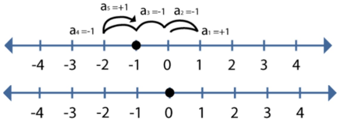
A classical random walk is a mathematical model that describes the movement of a particle in a series of discrete steps, where each step is chosen randomly from a set of possible directions. Visualized in Figure 1 as a particle takes steps in either a positive or negative direction along a one-dimensional line (possibly higher dimensions), the particle’s position is updated after each step through an equal coin toss, and the process continues for a specified number of steps [3].

Figure 1. (Bottom) The walker starts at “0” with no steps taken. (Top) The walker moves through each step of the random walk, with the 1st step a1, the second step a2, the third step a3 and etc. The “+1” represents a step to the right, while a “-1” represents a step to the left. Here, 5 steps have been taken and the final destination of the walker is at -1 on the line.

Quantum Random Walk.

Quantum random walk is an extension of, but also an advantage to classical random walk, in that it utilizes superposition and entanglement. In a quantum random walk, a particle exists in a superposition of multiple locations simultaneously, represented by quantum states. At each step, the particle’s state evolves through a unitary transformation, which in quantum mechanics corresponds to a rotation of axes in the Hilbert space that does not alter the normalization of the state vector but a change in different components. These transformations are facilitated through quantum operators, where the probabilities of transitioning to neighboring nodes combine either constructively or destructively for different quantum paths [4]. The vast use of quantum random walks stems from the fact that: Firstly, quantum random walks can exhibit faster spreading or localization compared to classical random walks. Quantum interference can concentrate the particle’s probability distribution in specific regions, leading to accelerated exploration or enhanced localization, depending on the setup. Secondly, quantum random walks can provide exponential speedups in certain algorithms and search problems via enhanced exploration, accelerated search, and exponential speedups in certain computational tasks [5].

The most important observation on quantum random walks is that in classical random walk, \(\sigma^2 \sim T\), where “\(\sigma\)” is the standard deviation of the random walk’s probability distribution, and “\(T\)” is the number of time-steps of the random walk. For the quantum random walk, it is instead \(\sigma^2 \sim T^2\), meaning the standard deviation grows at a quadratically faster rate per time-step.

More on the probability distributions as seen in Figure 2, the probability distribution of the classical random walk resembles most of a Gaussian distribution, since extreme positions from the starting node are less likely to happen in a stochastic model. However, in quantum random walk, the walker is allowed to travel separate directions at the same time because of superposition. With this, constructive/destructive quantum interference increases or decreases the probability of certain positions due to the overlap of different paths, thus producing a probability distribution that is more complex than that of classical random walk. Figure 2 shows how quantum random walk has a different probability distribution in final positions at different peaks than does classical random walk [6].

Figure 2. In classical random walk, the walker travels a single node per unit time in its stochastic model, while quantum random walk utilizes superposition for all the nodes’ states and applies unitary transformation through the particle’s evolution. Every arrow for each node represents a singular path taken in the classical random walk example, while the arrows for each node represent multiple paths taken simultaneously. The probability distributions of the final position of the walker is different in each of the random walks, as shown by the height of the orange bars.

Quantum Walk with Quantum Coin.

Within quantum random walk, there exists a quantum coin that guides the evolution of the quantum walker. This approach allows for more control and flexibility in manipulating the walker’s behavior. This coin represents a quantum system that can be prepared in a superposition of basis states. The evolution of the walker involves two main steps: the coin operation and the conditional shift operation. The coin operation applies a unitary transformation to the coin degree of freedom, while the conditional shift operation modifies the walker’s position based on the coin state. In a standard quantum random walk with a quantum coin on a line graph, the Hadamard gate (H) is often used as the coin operation [7]. Using the Hadamard gate as the quantum coin is just one of many gates that can be used in quantum walk. But the Hadamard gate, as represented by

\[H=\frac{1}{\sqrt{2}}\begin{bmatrix} 1 & 1 \\ 1 & -1 \end{bmatrix}\tag{1}\]

allows for equal probability distributed within the superposition. Applied to the coin qubit, the Hadamard gate creates a superposition of the basis states, leading to an equally balanced exploration of both left and right directions in subsequent steps of the walk, known as a plus state, which uses bra-ket notation:

\[|+\rangle=\frac{|0\rangle+|1\rangle}{\sqrt{2}}\tag{2}\]

MATERIALS AND METHODS.

Quantum random walks on entangled states are analyzed for two to six qubits. One way to represent these qubits is via a four-nodes graph as shown in Figures S1~S4. Quantum states of qubits are denoted as such:

\[|0\rangle=\begin{bmatrix} 1 \\ 0 \end{bmatrix}\tag{3}\]

\[|1\rangle=\begin{bmatrix} 0 \\ 1 \end{bmatrix}\tag{4}\]

There are two different types of entangled states: Greenberger-Horne-Zeilinger states (maximally-entangled states produced by the Hadamard gate through

\[|GHZ\rangle=\frac{|0\rangle^{\otimes n}+|1\rangle^{\otimes n}}{\sqrt{2}}\tag{5}\]

where an n-qubit GHZ state has the basis states \(|0\rangle^{\otimes n}\) and \(|1\rangle^{\otimes n}\) in Eq. 5, denoted as tensor products (\(\otimes\))), and partially entangled states. Unlike GHZ states, partially entangled states of two or more particles become correlated in such a way that the state of one particle cannot be described independently of the state of the other particle, even when separated. In another perspective, the measurements of GHZ states fully collapse to a single state, like \(|0\rangle\) or \(|1\rangle\). However, in partially-entangled states, the measurement does not necessarily destroy the entangled state of others. An example of such a partially-entangled state is \(\frac{|110\rangle+|101\rangle+|011\rangle}{\sqrt{3}}\) . If the first qubit of this state (where the first to third qubit is represented from left to right for each basis state), is measured and collapsed to \(|1\rangle\), the result is \(|1\rangle\otimes(|10\rangle+|01\rangle)\). The measurement can be represented as a tensor product of two or more states, with one of those states being a special entangled state for two-qubits (called a Bell state), \(|10\rangle\) + \(|01\rangle\). Thus, we find that after measurements of partially-entangled states, the result only partially collapses all the basis states.

As shown in Figures S1~S4, each node in the graphs (qubit) are labeled from A-D, where enclosed line around qubits represents a maximal-entanglement around the enclosed qubits. Figure S1 represents an entangled state of qubits A and B, which represents the simplest entanglement of qubits. In Figure S2, the lines encompass qubits A, C, and D, which is a 3-qubit entangled cluster. Subsequently, Figure S3 shows an entanglement between all four qubits. However, Figure S4 represents a partially entangled state, which only exhibit some degree of entanglement between the constituent quantum systems. They are not fully entangled in the representation of a graph, since more than one entangled cluster overlaps each other. Thus, graph 4 represents a combination of an entangled state between qubits A and B and a 3-qubit GHZ state with qubits A, C, D.

Although the quantum graphs are only visually represented with entangled states of up to four qubits, entangled states are analyzed up to six qubits. Over sixty different combinations and hundreds of different permutations of possible superposition states for two to six qubits were analyzed; with such variety, examples of different possible entangled states and other references for two to six qubits can be found on https://drive.google.com/drive/folders/17nE74v-2zp1Y6Rc0rfbeo‌ECo41yBX6LH?usp=sharing.

As a representation of quantum states, quantum circuits are created using different gates. The simplest of these to create are the GHZ states. In Figure 3, the top circuit shows a representation of a GHZ state of two qubits while the bottom circuit represents a GHZ state of 5 qubits using the Hadamard gate and CNOT gate(s), which are two-qubit quantum gates that flip a target qubit if and only if the control qubit is in the state \(|1\rangle\) using the matrix representation \(\begin{bmatrix} 1&0&0&0\\ 0&1&0&0\\0&0&0&1\\0&0&1&0 \end{bmatrix}\).

Figure 3. Quantum circuits created on IBM Quantum Composer in this study. Every gray line on a quantum circuit denotes a position of a qubit, as listed by indices starting at 0 (q[0], q[1],…etc.). Each qubit starts initially with a state of |0>, and are manipulated by adding quantum gates to qubit(s): The “H” gate represents the Hadamard gate, the “+” gate represents the CNOT gate, and the gray boxes represent measurements of each qubit, which are represented as arrows pointing down to c(n), where n is the number of qubits.

For non-GHZ states, the process is more complex. Though GHZ states can be created with just Hadamard and CNOT gates, non-GHZ states, which can be factored by a \(|0\rangle^{\otimes n}\) or \(|1\rangle^{\otimes n}\), require the use of NOT (performs a bit flip on a qubit through the configuration \(\begin{bmatrix} 0&1\\ 1&0 \end{bmatrix}\)) and Z gates (performs a phase shift on a qubit but leaves the basis states \(|0\rangle\) and \(|1\rangle\) unchanged through the configuration \(\begin{bmatrix} 1&0\\ 0&-1 \end{bmatrix}\)). The process for finding all the non-GHZ states starts with choosing the number of qubits used and the number of basis states for the entangled state (Within the scope of this study, only superposition states that contained an even number of basis states were considered). If, for example, the conditions are five qubits with four basis states, a possible entangled state under those conditions is chosen. One example is the state represented in Figure S5: \(\frac{|10000\rangle+|01000\rangle+|00100\rangle+|00011\rangle}{\sqrt{2}}\). Then, combinations of applying NOT and Z gates on different qubit locations over the particular superposition state are produced and measured. An example of a combination is by applying a NOT gate to every second and third qubit in the circuit for Figure S5 as shown in Figure S6, or a Z gate to the fourth qubit of each basis state in Figure S7. After listing out all possible entangled states from two to six qubits in this manner, all the states were created and visually represented via the quantum IBM composer to create the quantum circuits, get the probability distribution of the basis states in each superposition, and receive the number of actual outputs of basis states in each superposition state.

RESULTS.

After running the measurements for all the entangled states and those associated with the quantum random walks on the GHZ states on 1,024 shots (measurements), there were two main results: When measuring the outputs of each of the basis states for the entangled states, there was no clear pattern shown on what would give the most outputs for one basis state. Instead of a conclusion, there can only be observations based on the measurements for the entangled states. For example, Figure 4 shows a histogram of the number of frequencies for each of the basis states illustrated in Figure S8:

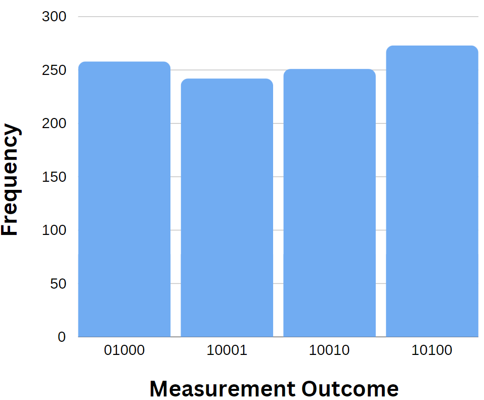
Figure 4. Quantum circuit and graph created on IBM Quantum Composer. Out of 1,024 shots (measurements of the superposition), the frequency output of individual basis states |0100>, |10001>, |10010>, and |10100> are recorded.

There are 258 outputs for \(|01000\rangle\), 242 outputs for \(|10001\rangle\), 251 outputs for \(|10010\rangle\), and 273 outputs for \(|10100\rangle\). These results can be shown for all entangled states in another place. In addition, when starting on a different qubit on the quantum random walks for 3 to six qubits, the outputs of each of the basis states were not the same and unique as just measuring the entangled states. However, almost all of the quantum random walks had the most outputs on either \(|0\rangle^{\otimes n}\) or the basis state \(|1\rangle^{\otimes n}\), which are found in the basis states of GHZ states, where n is the number of qubits used in the quantum random walk. The only exception in the measurements were two quantum circuits with five qubits, shown in Figure S9 which showed the highest output on the basis state \(|11011\rangle\), and Figure S10, which showed the highest output on the basis state\(|00100\rangle\).

DISCUSSION.

The goal of this study was to explore the entangled states, their representation on quantum graphs, and applications of quantum random walk over GHZ states. The results demonstrate that by measuring quantum random walk with a quantum coin on the GHZ states, the basis states that have the most output are mainly the basis states that come from the GHZ states themselves, although there wasn’t a clear obvious pattern for which basis state had the most frequent output. However, one can conclude that information stored in each qubit of the basis states that resemble those of the GHZ basis state may have the highest probability in yielding results when measured. This information may be useful, since quantum basis states that either store all 0’s or all 1’s (or in different contexts, all yes’s or all no’s) on average are more likely to happen when measured using quantum random walk. One thing for certain is that the measurement results are derived from more computational power on quantum versions of random walk, which shorten the amount of time and space to run computations of a given path position across graphs. Specifically, the idea that superpositions allow for quantum walks to travel multiple paths through a graph simultaneously while classical random walks only allow a walker to travel a single path at a time, supports the fact that quantum computation offers high potential in random walk applications.

Limitations for this analysis include that not all non-GHZ states created on the quantum composer were considered and that the methods only covered non-GHZ states with even numbers of basis states in its superposition. Due to the overwhelming complexity of non-GHZ states with odd-number basis states, they are not included in this study. In addition, future research can delve into the possibilities of quantum graphs and quantum random walks with systems containing more than six qubits. Other factors may be tested, such as analyzing more than six qubits due to the nature of exponential growth of possible entangled states, or using different coin registers for the quantum random walk. Instead of a Hadamard coin, one could use the Grover coin, or other shift operations that alter the freedom of the walker throughout each step. The number of shots used to record the output frequencies for the different basis states could’ve been more than 1,024 or less than 1,024 shots used as well. These factors could possibly produce a more consistent, spontaneous pattern of basis states that tend to receive the most output when measured.

Altogether, these experiments are possible through the properties of quantum computation, allowing for discoveries in search algorithms, optimization problems, simulations, and machine learning. As shown by the advantages of quantum random walk, such quantum algorithms may contribute to the development of algorithms that leverage entanglement to explore solution spaces in a manner that surpasses classic algorithms, leading to a potential speedup in problem-solving. For example, new discoveries in quantum random walks may play a role in enhancing the security and efficiency of quantum communication that focuses on the secure transmission of information using the principles of quantum mechanics. Thus, the possibilities of quantum walk behavior should be further analyzed for the advancement of less-cost, efficient systems.

SUPPORTING INFORMATION.

Supporting Information includes Entangled Graph Diagrams for Partially-Entangled States and Quantum Circuits for Corresponding Entangled Circuits in the Materials and Methods.

ACKNOWLEDGMENTS.

I would like to thank and appreciate Post-Doctoral Researcher Fatimah Ahmadi Rita and the Lumiere Team for helping facilitate research in this project and for other high school students in research.

REFERENCES.

B. Hensen, H. Bernien, A. E. Dréau, Reiserer, N. Kalb, M.S. Blok, J. Ruitenberg, R.F.L. Vermeulen, R. N. Schouten, Experimental loophole-free violation of a Bell inequality using entangled electron spins separated by 1.3km. Nature. 526, 682-686 (2015).
J. Preskill, Quantum computing in the NISQ era and beyond. Quantum. 2, 79 (2018).
G. H. Weiss, Aspects and applications of the random walk. Journal of Statistical Physics. 79, 497-500 (1995).
N. Shenvi, J. Kempe, K. B. Whaley, A Quantum Random Walk Search Algorithm. Physical Review A. 67, 052307 (2003).
A. Ambainis, Quantum walks and their algorithmic applications. International Journal of Quantum Information. 1, 507-518 (2003).
A. M. Childs, J. Goldstone, Spatial search by quantum walk. Physical Review A. 70, 022314 (2004).
S. E. Venegas-Andraca, Quantum walks: a comprehensive review. Quantum Information Processing. 11, 1015-1106 (2012).

Posted by buchanle on Tuesday, April 30, 2024 in May 2024.

Tags: Entangled States, Quantum Circuit, Quantum Coin, Quantum Computing, Quantum Random Walk