Developing cheaper and safer non-weather-based AI models for microgrid demand and supply forecasting in rural areas
ABSTRACT
A number of studies have used various machine learning (ML) techniques to forecast the demand (load) and supply (power production) of microgrid power in rural areas, using weather data as inputs; however, there are many practical problems with this data. This includes exorbitant procurement costs and a dearth of communication-failure backups with weather data services. The current literature has not yet addressed these pragmatic concerns. These problems also make the implementation of microgrids and the widespread deployment of solar power more challenging, especially in rural areas with low-income levels. As a more practical alternative to weather-based models, this study suggests models that instead use historical data of power demand and supply. We employ ML techniques using historical data to forecast demand and supply over five different time horizons: 15 minutes, 1-hour, 1-day, 1-week, and 1-month. Demand-side and supply-side forecasting performs best using the Linear Regression model, which also had the best Pearson Correlation Coefficient, Mean Absolute Error and Root Mean Squared Error—comparable to state-of-the-art weather-based models. Our models are a cheaper and safer option—enabling wider deployment of microgrids and solar power in rural areas, especially where high costs are an issue.
INTRODUCTION.
Access to energy is an essential catalyst for socioeconomic development in rural areas. A growing number of people in rural areas now have access to electricity thanks to microgrid solutions, where the national grid often does not provide electricity. Developers of microgrids must manage their current locations and extend to new areas (1). On the other hand, in certain rural areas, an increasing number of microgrids have begun to diversify their power supply by including renewable energies. The design of a new power management system is necessary for the integration and optimization of the various energy sources. This system must be able to predict how much electricity the community will use and how much electricity will be produced from renewable sources in order to manage the fossil fuel-based generators and satisfy the community’s power needs (2).
Furthermore, in rural areas in developing countries such as Bangladesh, the government is unable to provide enough support for national grid extension and distributing energy to remote rural areas due to high investment and maintenance costs (3). Hence, microgrids are the only way to access electricity. However, the high costs of forecasting (demand and supply) and unreliability of a microgrid, especially when run on solar photovoltaic (PV) cells, makes implementing a microgrid in rural areas difficult as well (3).
In the literature, a number of machine learning (ML) and artificial intelligence (AI) forecasting models have been proposed for microgrid developers, in order to reduce the unreliability of running a microgrid and to create a ‘power management system’: the load or consumers’ consumption (‘demand-side’) must be predicted; the power production by the solar PV cells (‘supply-side’) must be predicted as well (1).
Otieno et al. successfully forecasted energy demand for microgrids over multiple horizons in Sub-Saharan Africa, with the best forecasts using an exponential smoothing technique (1). Mcsharry et al. also successfully forecasted energy demand, but using a probabilistic approach, with a key outcome of the paper in identifying the needed time-horizons for microgrid developers. They identify three particular ‘time-horizons’: (1) very short-term forecasting (minutes to hours), (2) short-term load forecasting (hours to weeks), and (3) medium-term to long-term forecasting (weeks to months to a year) (4). Cenek et al. applied long short-term memory (LSTM) and artificial neural networks (ANNs) to the problem, working to forecast load in rural areas in Alaska, using a relatively small amount of training data to achieve a high accuracy (2).
On the other hand, when it comes to power supply forecasting, various studies have also had success in the area. For instance, in the literature review of Mosavi et al., various studies with success are identified that use a wide array of statistical and ML approaches for forecasting power supply (5). Many studies also attempt to predict solar irradiation (which directly correlates with solar power production), such as Ahmad et al.’s models in predicting solar radiation one-day-ahead in New Zealand using commonly-used time-series models like Multilayer Perceptron (MLP), Nonlinear Autoregressive Network with Exogeneous Inputs (NARX), Autoregressive Integrated Moving Average (ARIMA), and persistence methods (6).
However, other successful state-of-the-art models cited by Mosavi et al. all use weather data as inputs (5). Ordiano et al. points out the problem with using this type of data. They note exorbitant costs associated with purchasing weather data on an hourly or even minute-to-minute basis to run these forecasting models, as specific types of data—such as solar radiation in a specific area of a solar farm—are not available free-of-charge to microgrid developers. They also note that in case of communication failures with weather data services, the forecasting models would fail to run, causing failure of the entire power management system (a high risk). Hence, Ordiano et al. proposed using non-weather-data, such as high-resolution and highly-granular past-power production data, to predict future power production data: removing all data costs and reducing communication-failure risk, being the cheapest and safest option (7).
Ordiano et al. achieved success with their supply-side forecasting models (7). Inspired by their study, the goal of this study is to apply their method to bothdemand-side and supply-side forecasting, but more specifically, with microgrid developers in rural areas in mind. By increasing the reliability and cost of running a microgrid in rural areas, the goal of this study is to help increase access to electricity and renewable energies in rural areas. As such, we will be testing our models on 31 datasets (various locations across the same microgrid) in order to test and ensure model robustness across the board. We hypothesize that if we use the past power supply and demand data to predict the future power supply and demand, then we would achieve a high accuracy, as the past power supply and demand data are highly correlated with the weather-data, which would make our non-weather-based models still highly accurate, but cheaper and more reliable.
MATERIALS AND METHODS.
Original dataset – UCSD microgrid data. We used the dataset ‘Open-Source Multi-Year Power Generation, Consumption, and Storage Data in a Microgrid’, published by Silwal et al. (8). It consists of “open-source, high resolution” data on power consumption and production from the University of California, San Diego (UCSD) microgrid. The microgrid has “several distributed energy resources (DERs)”. The resolution of the data was 15-minutes. We only used the ‘real power’ and omitted the ‘reactive power’ and ‘date and time’ column. This left the dataset with only one column: ‘real power.’ We used data from all five years of the dataset, from 1st January, 2015 to 29th February, 2020. We tested our ML techniques on all 16 locations of the demand data available in the dataset inside the UCSD campus, and all 25 locations of the supply data available also.
Transformation of the dataset. We transformed the dataset from the original based on the resolution. For example, for the 15-minute-resolution, we first duplicated the original ‘real power’ column of the dataset. Then, we shifted the second ‘real power’ column up by one row. This made the first ‘real power’ column the historical data column (the feature), and the second ‘real power’ column the future predicted data column (the target). This was done for the other resolutions as well, particularly the 1-hour resolution (where the power was predicted for every 15 minutes in the predicted hour; hence there were four target values in the 1-hour resolution). For the 1-day, 1-week, and 1-month resolution, this method was adjusted slightly. For the 1-day prediction, we predicted this with 24 targets (hourly resolution); for the 1-week prediction, with 7 targets (daily resolution); for the 1-month prediction, with 30 targets (daily resolution). We summed the values in the original dataset for these adjusted predictions; for example, for the 1-day-ahead prediction with 24 targets (hourly resolution), we summed every four columns in the original dataset together to form a new dataset with hourly resolution. Then, as before, the process of duplicating the ‘real power’ column (now of hourly resolution) occurred. However, it occurred differently for each different prediction set. For example, for the 1-day-ahead prediction, the new hourly resolution dataset was duplicated 47 times, and shifted 47 times up as well, so that the dataset in total would have 48 columns. Of these 48, the first 24 were the historical data of the past 24 hours (input data), the second 24 were the future data of the next 24 hours (target data). This is how ultimately later the dataset was split as feature and target.
Shape of the dataset.
On average, the original 16 demand datasets had 141,258 rows and the original 25 supply datasets had 139,290 rows.
Machine learning algorithms. Due to the large size of each dataset (and as we had to run each model on a total of 31 datasets) the size of the tasks of this paper were quite computationally intensive. Due to a lack of computational resources available, we only test four simple models with their default parameters in the sci-kit learn library: Linear Regression (LR), K-Nearest Neighbors (KNN), Decision Tree (DT), and Random Forest (RF). However, despite trying quite simple models, the robust dataset meant that a large amount of training data was available—which improved the results of the models significantly.
All four models are quite commonly used throughout machine learning, and are examples of supervised learning (where labelled data is used to predict an outcome, as opposed to unlabeled data in unsupervised learning). RF utilizes multiple decision trees (a tree-like model of event outcomes and their probabilities), combining all their outputs to reach a final result. In comparison, DT is simply a graph with all the possible outcomes of a decision (one decision tree). The latter (DT) is much easier to visualize than the former (RF) and much faster to run as well since it only uses one decision tree; while RF, even though slower, tends to be more accurate and precise (and has less overfitting) as it combines the results of multiple decision trees (and is harder to visualize as it has so many trees).
Meanwhile, LR works by using a linear equation: using the independent value directly to predict the dependent value. The goal is to optimize the coefficients of the linear equation (minimize the distance between the predicted and actual value, or the ‘error’), so the ‘best-fit’ line predicts the dependent values accurately and without overfitting. There may be multiple independent variables (hence multiple coefficients) in the linear equation. The main advantage of LR is that it is fairly simple and easy-to-interpret.
A KNN model on the other hand works differently from classification to regression. The basic assumption in classification is that the outcome most-represented in the k-nearest neighbors around the point (where k is an integer greater than 0) is used to predict that point’s outcome. This assumption carries over in regression: an average of the k-nearest neighbor points is taken to predict the outcome of the point. To find the ‘nearest’ neighbors, different types of distance can be measured; but Euclidean distance is the most commonly used. The main advantage of KNN is that it has no training time as all the dataset’s points are used when making predictions; but, the optimal value of k does need to be determined through testing.
Data splits. The data was split with a ratio of 90-10 between the training and testing. A validation set was not used as the models were tested on not one, but 31 separate datasets, which should indicate model robustness across a variety of locations’ production and consumption patterns.
Evaluation Metrics. Three key metrics are measured: the Pearson Correlation Coefficient (PCC), the Mean Absolute Error (MAE), and the Root Mean Squared Error (RMSE). In essence, PCC measures the strength of the relationship between two variables (in our case, between the predicted value and the actual value). All our correlations are positive, so a PCC value of 0 would mean no correlation, and 1 would mean total positive correlation. MAE and RMSE are different measures of the errors (the differences between the predicted value and the actual value). MAE and RMSE’s values are often interpretable as they as in the same unit as the dataset. RMSE penalizes outliers and larger errors more than MAE (as RMSE squares them). For both RMSE and MAE, the lower the value, the more accurate the model is (and values range from zero to infinity). If MAE is too simplistic to understand a dataset (and it is desired to get rid of the larger outliers in the data) then RMSE is usually used.
In our case, we use PCC to compare our results with other state-of-the-art studies, as PCC does not have any units and can be compared across studies. On the other hand, MAE and RMSE are in the units of our dataset’s target value (kilowatt-hours), so those metrics can only be used to compare the performance of different models within our study relative to each other (but no cross-study comparisons).
Equation 1 indicates the error in forecasting, where represents the forecasting error, k represents the time sample, \(\hat{P} [k]\) represents the predicted value, and \(P[k]\) represents the actual value:
\[e_f\left[k\right]=\ \hat{P}\ [k] – P [k]\tag{1}\]
Equation 2 represents the PCC equation, where \(r_{P\hat{P}}\) is the PCC, K represents the total number of samples, \(\bar{P}\) and \(\bar{\hat{P}}\) represent the averages of each respective time series:
\[r_{P\hat{P}}=\ \frac{\sum_{k=1}^{K}{\left(P\left[k\right]-\bar{P}\right)\ (\hat{P}\left[k\right]-\bar{\hat{P}})}}{\sqrt{\sum_{k=1}^{K}\left(P\left[k\right]-\bar{P}\right)^2}\ \ \ \ \ \sqrt{\sum_{k=1}^{K}{(\hat{P}\left[k\right]-\bar{\hat{P}})}^2}}\tag{2}\]
Equation 3 represents the MAE equation:
\[MAE\ =\ \ \frac{1}{K}\sum_{k=1}^{K}\left|e_f\left[k\right]\right|\tag{3}\]
Equation 4 represents the RMSE equation:
\[RMSE = \sqrt{\frac{1}{K}\sum_{k=1}^{K}{(e_{f}[k]^2)}}\tag{4}\]
RESULTS.
Table 1 shows the results for both demand-side and supply-side forecasting for all three metrics (PCC, MAE, RMSE).
| Table 1. Results for both demand-side and supply-side forecasting. Results are shown for four models (LR, KNN, DT, RF), three metrics (PCC, MAE, RMSE), and five time horizons (15 min ahead, 1 hour ahead, 1 day ahead, 1 week ahead, and 1 month ahead). | ||||||
| AI Model | Metric | Forecasting Time Horizons | ||||
| 15 min ahead | 1 hour ahead | 1 day ahead | 1 week ahead | 1 month ahead | ||
| Demand-side forecasting | ||||||
| LR | PCC | 0.97 | 0.95 | 0.97 | >0.99 | >0.99 |
| MAE | 16.42 | 17.33 | 16.75 | 11.33 | 1105.55 | |
| RMSE | 19.01 | 20.72 | 19.23 | 12.40 | 1219.49 | |
| KNN | PCC | 0.95 | 0.93 | 0.92 | 0.91 | 0.86 |
| MAE | 15.15 | 14.99 | 13.15 | 12.24 | 1005.52 | |
| RMSE | 17.60 | 18.06 | 15.76 | 14.83 | 1219.27 | |
| DT | PCC | 0.90 | 0.90 | 0.95 | >0.99 | >0.99 |
| MAE | 16.01 | 15.79 | 15.57 | 11.34 | 1100.37 | |
| RMSE | 18.81 | 19.49 | 18.99 | 12.43 | 1210.70 | |
| RF | PCC | 0.92 | 0.93 | 0.96 | >0.99 | >0.99 |
| MAE | 17.61 | 14.81 | 14.40 | 11.34 | 1104.30 | |
| RMSE | 18.26 | 17.88 | 16.42 | 12.42 | 1216.44 | |
| Supply-side forecasting | ||||||
| LR | PCC | 0.98 | 0.96 | >0.99 | >0.99 | 0.99 |
| MAE | 4.09 | 5.13 | 3.35 | 2.62 | 225.81 | |
| RMSE | 6.95 | 8.45 | 5.45 | 4.23 | 257.42 | |
| KNN | PCC | 0.98 | 0.97 | 0.99 | 0.98 | 0.87 |
| MAE | 4.36 | 5.54 | 3.05 | 2.73 | 343.44 | |
| RMSE | 7.12 | 8.66 | 5.43 | 5.41 | 413.18 | |
| DT | PCC | 0.97 | 0.94 | 0.94 | 0.90 | 0.56 |
| MAE | 4.34 | 5.53 | 4.15 | 4.43 | 226.17 | |
| RMSE | 7.22 | 8.83 | 7.42 | 8.74 | 256.90 | |
| RF | PCC | 0.97 | 0.94 | 0.97 | 0.95 | 0.80 |
| MAE | 4.69 | 6.03 | 3.34 | 3.23 | 224.89 | |
| RMSE | 7.65 | 9.18 | 5.63 | 6.07 | 256.22 | |
Demand-side vs. supply-side forecasting. As per Table 1, between demand-side and supply-side forecasting, the supply-side forecasting shows better results. Although the PCC values were mostly within the same range for both demand-side and supply-side, the MAE and RMSE reveal more insights. Consistently, the demand-side forecasting has a higher MAE and RMSE, indicating higher error. For example, for the 1-month-ahead forecasts, the demand-side MAE and RMSE values are almost five times higher than the supply-side values. A possible reason for this is that while the past power supply (power production) data is a highly-correlating substitute to the weather data used in weather-based models, the past demand data still may be highly volatile.
Forecasting time horizons. Consistently, the 1-month-ahead forecasts performs the worst, with the highest RMSE and MAE. Then, from worst to best-performing in terms of RMSE and MAE are 1-hour- ahead, 15-min-ahead, 1-day-ahead, then 1-week-ahead (however, between these four forecasting horizons, the error differences are not extremely large). These results indicate that while the 15-min ahead, 1-hour-ahead, 1-day-ahead, and 1-week-ahead forecasts from our models may be usable, the 1-month may not be due to the large errors.
Highest-scoring vs. lowest-scoring models (using MAE and RMSE). Consistently, the best-performing model for nearly all metrics, especially the PCC was LR. The worst-performing model for nearly all metrics was RF (although the biggest differences between RF and the rest of the models was only observed for PCC, not MAE and RMSE). On the other hand, DT is much worse than KNN for supply-side forecasting (with the worst PCC value of 0.56 in the monthly forecast), and KNN is worse than DT for demand-side forecasting (PCC of 0.86 for KNN, compared to PCC of almost 1 for DT, for the monthly forecast).
Comparison to state-of-the-art weather-based models (using PCC). To make cross-study comparisons, the PCC value is used. In the state-of-the-art models’ literature review by Mosavi et al., the best and most competitive weather-based models have a PCC ranging from 0.96 to almost 1 (5). For our best model, LR, for all time-horizons we are within that range for the PCC, with the exception of the 1-hour-ahead forecast for demand-side forecasting which has a PCC value of 0.95. However, the rest of our models are also competitively within or quite close to that range of weather-based models, indicating that our approach, especially using LR, can be a suitable substitute for almost all of the time horizon forecasts to weather-based models.
Example forecast of supply-side forecasting: LR, 15-minutes-ahead. Figure 1 shows an example forecast using our best model, LR, for the 15-minutes-ahead time horizon.
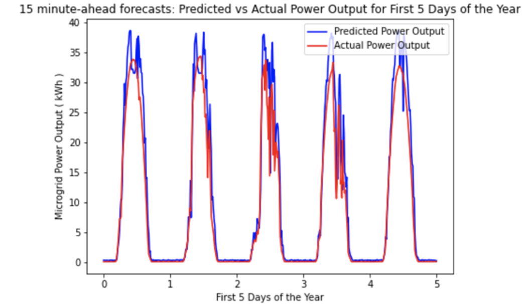
Figure 1. 15-minute-ahead forecast example using LR: Predicted vs Actual Power Output for the First 5 Days of the Year. The figure indicates that our model performs relatively well during most hours of the day, except for ‘middle of the day’ where more volatility is seen in the dataset. Between day 4 and day 5, for example, although actual power output was relatively smooth, our model predicts more volatility. Between day 2 and 3, our model overestimates the power production, despite catching the volatility. Hence, this shows that even though our PCC for this forecast is quite high (0.98), our model does not overfit.
DISCUSSION.
We hypothesized that if we use the past power supply and demand data to predict the future power supply and demand, then we would achieve a high accuracy, as the past power supply and demand data are highly correlated with the weather-data, which would make our non-weather-based models still highly accurate—but cheaper and more reliable. Our hypothesis was shown to be mostly true, especially as our accuracies for our best model, LR, were comparable to state-of-the-art models cited in the literature review by Mosavi et al. (5).
The main limitations of this study will now be addressed. The demand-side forecasting was shown to be less accurate than the supply-side forecasting, and ‘middle of day hours’ (where there was high volatility) was less accurate as well. Adding ‘time of day’ of ‘time of year’ data to our models may improve this, as consumers’ demand and volatility are highly correlated with particular times of the day as well. Exploring further avenues of ML, such as feature engineering, or other complex time series models such as ARIMA may also help this. Furthermore, the monthly forecasting time horizon also did not perform well. In this case, weather-based models such as those of Otieno et al., Mcsharry et al., and Cenek et al. can be used, as those only require purchasing weather data 12 times a year (which is a low cost, compared to purchasing it every 15 minutes a year) (1, 2, 3).
However, the comparable PCC values to state-of-the-art models, and robustness of results (as these metrics were tested across 31 datasets) indicate the strength of these non-weather-based models as cheaper, more reliable substitutes—enabling wider deployment of microgrids and solar power in rural areas especially, where high costs are an issue.
ACKNOWLEDGMENTS.
Thanks to the Lumiere Research Scholar Program for allowing us to do this work!
REFERENCES
- F. Otieno, N. Williams, P. McSharry, Forecasting Energy Demand for Microgrids Over Multiple Horizons. IEEE Xplore (2018), pp. 457–462.
- M. Cenek, R. Haro, B. Sayers, J. Peng, Climate Change and Power Security: Power Load Prediction for Rural Electrical Microgrids Using Long Short Term Memory and Artificial Neural Networks. Applied Sciences. 8, 749 (2018).
- M. Shoeb, GM. Shafiullah, Renewable Energy Integrated Islanded Microgrid for Sustainable Irrigation—A Bangladesh Perspective. Energies. 11, 1283 (2018).
- P. E. McSharry, S. Bouwman, G. Bloemhof, Probabilistic Forecasts of the Magnitude and Timing of Peak Electricity Demand. IEEE Transactions on Power Systems. 20, 1166–1172 (2005).
- A. Mosavi, M. Salimi, S. Faizollahzadeh Ardabili, T. Rabczuk, S. Shamshirband, A. Varkonyi-Koczy, State of the Art of Machine Learning Models in Energy Systems, a Systematic Review. Energies. 12, 1301 (2019).
- A. Ahmad, T. N. Anderson, T. T. Lie, Hourly global solar irradiation forecasting for New Zealand. Solar Energy. 122, 1398–1408 (2015).
- J. Á. González Ordiano, S. Waczowicz, M. Reischl, R. Mikut, V. Hagenmeyer, Photovoltaic power forecasting using simple data-driven models without weather data. Computer Science – Research and Development. 32, 237–246 (2016).
- S. Silwal, C. Mullican, Y.-A. Chen, A. Ghosh, J. Dilliott, J. Kleissl, Open-source multi-year power generation, consumption, and storage data in a microgrid. Journal of Renewable and Sustainable Energy. 13, 025301 (2021).

Posted by John Lee on Tuesday, May 30, 2023 in May 2023.
Tags: Artificial Intelligence, Machine learning, microgrid forecasting, renewable energy, rural areas