Determining the value of a cricket player: Does bowling ability have a greater effect on the rating of a cricket player than batting ability?

ABSTRACT

In this work, factors affecting the rating of a player in a cricket game were analyzed using the Pandas and Matplotlib libraries to discover patterns. Using a matrix correlation, a visualization technique reveals that only 7 out of the 15 variables in the matrix affected the rating. The predictive accuracy of linear regression, k nearest neighbors, and decision tree were compared, revealing that linear regression most accurately predicts the rating of a player (R-Squared value of 0.84). Further analysis of the data using linear regression shows that the most significant variables are the batting average of the player followed by the number of 50s the player has scored. This shows that the dataset used has a bias towards certain variables, indicating the need for optimization of any cricket dataset where machine learning is applied.

INTRODUCTION.

Sports and data have always gone hand in hand. In the past, coaches evaluated players based on their subjective interpretation of the player. The big data era has resulted in widespread access to large complex datasets. Also, the advancement of technology has improved modern data gathering and interpretation techniques, such as real-time video data capture. Sports analysts can now use potent algorithms to construct player strategies and game simulations for both minor and large matches. A paper on “Sports analytics and the big-data era”, reviews how the sports industry has been impacted by the rise in data availability and summarizes how the big-data era has presented unique research opportunities. It further provides examples of data-driven analyses that have impacted popular sports like baseball, basketball, and soccer. The paper concludes that less dynamic sports are easier to break down and analyze. Therefore, it shows that statistical approaches have been proven to yield better results in baseball when compared to basketball or soccer. Since cricket is a less dynamic sport than these, data analysis on cricket provides more reliable results than analysis on a more dynamic sport instead [1].

With easy access to many forms of data, the use of machine learning can enhance the use of data analysis in the sports industry. Large datasets make it possible to conduct original analysis to discover patterns between the variables that affect the value of a cricket player. Analysts can use various statistical methods to develop prediction models based on different variables.

For this research, the significance of the factors affecting the rating of a cricket player was analyzed. This relies on comparing the predictive accuracy of the different factors.

Effective prediction algorithms include regression and classification. Both are examples of supervised machine learning techniques in which a model is developed using correctly labeled datasets. The main distinction between classification and regression algorithms is that classification is used to predict or classify discrete values such as good player or bad player, True or False, safe, or not safe, etc., while regression algorithms are used to predict continuous values such as price, salary, height, etc.

Since the rating of a player is a continuous value, the use of classification methods is an ineffective approach to this task. Instead, the use of regression models will yield the highest predictive accuracy as it is more logical to predict an exact value for the rating of the player. Comparing the original rating to the predicted rating more easily shows which variables have the greatest impact on the rating than comparing the original rating to a categorized group such as “good player.”

The use of different regression models will build on previous research aimed at comparing data mining techniques. Cricket datasets tend to have many columns, each representing a variable that affects a player’s performance. These datasets give equal weight to the columns and assume that they all affect the performance of a player equally. This causes machine learning algorithms to produce biased results.

MATERIALS AND METHODS.

The data used came from Kaggle [8], a Google-owned data science community platform that ran ML-based prediction competitions utilizing databases that were accessible to the public. The dataset contains both the bowling and batting statistics of over 1700 cricket players and gives each player a rating. The dataset contains no text-based columns, so there is no need to introduce dummy columns. No pre-processing techniques have been implemented. Since there were no null values in the data, no observations had to be removed from the data; every player in the dataset was analyzed.

Definition of key variables in the dataset. The Age variable gives the age of the player as of 2018. Innings is the total number of matches in which the player has batted. The 100s and 50s variables give the total number of innings (matches) in which the players scored at least 100 runs and 50 runs respectively. The 6svariable is the total number of 6s that the player has hit (the most runs that can be scored in a single ball). Balls faced is the total number of balls that the player has faced as a batsman. Bat_Average is the batting average of the player – the average number of runs scored as a batsman. Runs scored is the total number of runs the player has scored as a batsman.

Balls bowled and overs bowled give the total number of balls and overs the player has bowled, there are six balls in one over. Bowl_Strike_Rate is the bowling strike rate, the number of balls the player has bowled per the number of wickets he has taken over his whole career, as a bowler. Maidens are the number of overs in which the player did not give away any runs when bowling. Wickets are the total number of times the player has dismissed a batsman (got him out) when bowling. Economy_Rate is the average number of runs the player has conceded per over bowled when bowling.

The rating column in the dataset was used to determine the value of the player and the factors that affect the rating. Different data mining and data visualization techniques were used to conduct the research and to find the correlation and hidden relationships between the variables. Therefore, it was logical to determine which data technique provides the most accurate results. Various Python libraries such as Num Py and Pandas were used for the analysis, Matplotlib for the visual representation of the data, and Seaborn and Sklearn for the machine learning.

The machine learning techniques used:

Linear regression. A linear approach for modelling the relationship between a scalar response and dependent and independent variables. It is a technique that is used to find the line of best fit that summarizes the relationship between the independent and dependent variables. The line of best fit is used to make predictions about the dependent variable based on new values of the independent variable.

K-nearest neighbor classifiers (KNN). A non-parametric, supervised learning classifier, which uses proximity to make classifications or predictions about the grouping of an individual data point.

It works by storing all of the available data points and classifying new data points based on their similarity to the stored data. In the KNN algorithm, the value of K determines the number of nearest neighbors used to make a prediction. For example, if K=3, the algorithm would find the three closest data points to the new data point and base its prediction on the majority class of those three neighbors. The idea behind the k-NN algorithm is that similar data points will likely have the same class label.

Decision Tree. A supervised learning approach that can be used for classification as well as regression. It uses a flowchart like a tree structure to show the predictions that result from a series of feature-based splits.

A decision tree is constructed by recursively splitting the data into subsets based on the values of the input features, until a stopping criterion is reached. Each node in the tree represents a test on a feature, and each branch represents the outcome of that test. The final leaves of the tree represent the predicted class or numeric value for a given observation.

The data visualization techniques used:

Correlation matrix. A useful tool for visualizing and summarizing the patterns in the data. The main use of the correlation matrix is to identify which variables affect the rating of a player. Using the information provided by the correlation matrix, a better idea about the relevant factors affecting the outcome can be achieved. Hence, the number of independent variables will be shortened to the most relevant ones.

Scatter plot. A graph to visualize the relationship between two numeric variables. The plots were used to visualize the relationship between each of the significant independent variables and the rating, for the top 15 players. The analysis of the top 15 players will give an insight into whether there is a visible pattern for the most valued players and whether it corresponds with the rest of the data.

Histogram and box plot. Visual representations of the distribution of the data. Since the rating is the dependent variable, its distribution will help me decide the ideal number of nearest neighbors for the KNN algorithm.

RESULTS.

From Figure 1 it can be concluded that both bowling and batting factors have an impact on the rating of a player. There are five batting factors and two bowling factors that have a significant positive correlation with the rating. Figure 1 shows that each of the five batting variables are correlated with one another and so are the two bowling variables. The batting variables used to ensure the most accurate results are 50s, 6s, Balls Faced, Bat_Average, and Runs scored. The bowling variables are Overs bowled and Balls bowled.

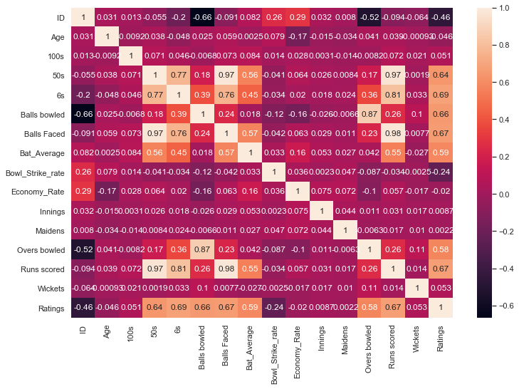
Figure 1. A correlation matrix that displays the correlation between all possible pairs of variables in the table [7]. The darker the color the higher the correlation.

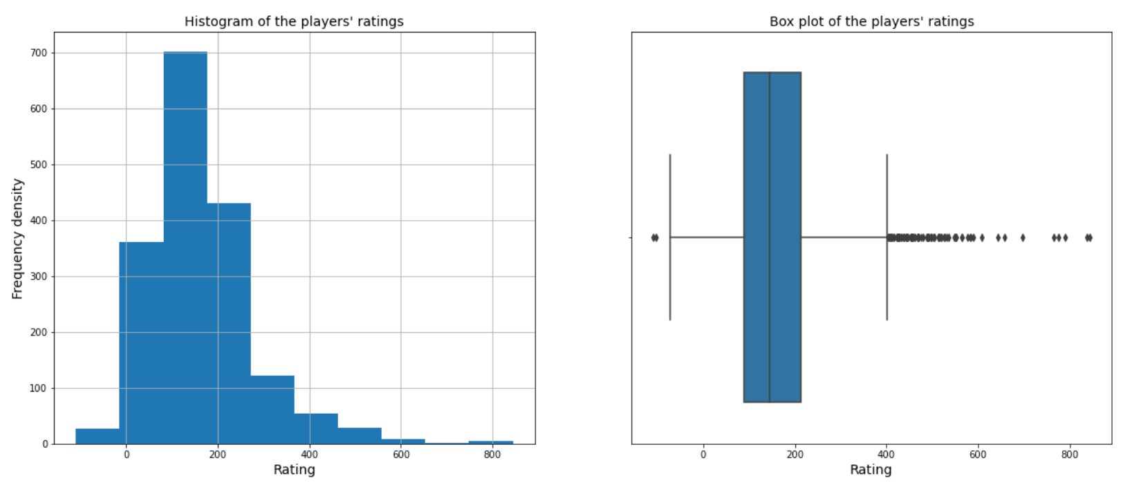
Figure 2 shows that the histogram is heavily skewed to the left, indicating most values are small, but there are a few exceptionally large ones. Those exceptional values will influence the mean and pull it to the right, causing the mean to exceed the median.

A B

Figure 2. The distribution for the rating column, shown through a histogram and box plot. Both show that the data is heavily skewed left i.e., the data mainly contains small values. The boxplot (B) can better highlight outliers in the data since it shows the median and quartiles of the data, whereas the histogram (A) only shows the shape and frequency distribution of the data.

A B

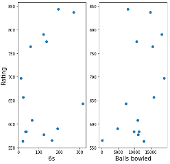
Figure 3. The most significant batting variable and the most significant bowling variable (based on correlation matrix) plotted for the top 15 players by rating. The x axis shows the different variables, and the y axis shows the rating. (A) The most significant batting variable and (B) the most significant bowling variable.

Figure 3 shows that the top 15 players are a mix of very good bowlers and batsmen. Despite there being more batting variables that affect rating than bowling variables, the bowling variables individually show a better correlation with the rating of a player. Since Figure 2 shows that the distribution for the rating is heavily skewed to the left, the results for the top 15 players are all outliers and they may not apply to the rest of the data.

To determine the accuracy of the machine learning algorithms, the R-squared value and mean square error for each algorithm were compared. The Mean squared error (MSE) represents the error of a predictive model created based on the given set of observations in the sample [8]. It is the sum of the squared difference between actual values and the predicted/estimated values divided by the total number of records. The R-Squared value [10] is a statistical measure of fit that indicates how much variation of a dependent variable is explained by the independent variable(s) in a regression model.

Results for the machine learning algorithms. When the linear regression model was applied to the data, the MSE is 2189.3319 and the R-Squared value is 0.8421. The Decision Tree model yielded a MSE of 3024.1183 and a R-Squared value of 0.7819. The K nearest neighbors model returned a MSE of 3659.3486 and a R-Squared value of 0.7384.

The results from the linear regression model give the most accurate results since the R-squared value is the highest and the mean square error is the lowest (MSE = 2189.3319 and R-Squared value = 0.8421). Therefore, the significance of the variables was determined using the linear regression model.

Table 1 shows the impact of each variable on the rating for the linear regression model. show that the most significant variable affecting the rating of a player is the batting average (Bat_Average) followed by 50s scored. The other variables all had a similar but low impact on the rating of a player. Balls faced was the only variable with a negative correlation. The condition number is large, 1.54e+03. This might indicate that there is strong multicollinearity (where several independent variables in a regression model are highly correlated) or other numerical problems [9].

Table 1. Results of in-depth linear regression.
Variable	Correlation with rating
50s	2.1051
6s	0.4436
Balls bowled	0.0311
Balls Faced	-0.0063
Bat_Average	5.5017
Overs bowled	0.0311
Runs scored	0.0068
*Condition number: 1.54e+03

DISCUSSION.

The histogram in Figure 2 shows 8 distinct blocks where the values for player rating have been distributed into. Hence, for the KNN algorithm, 8 nearest neighbors were the optimal number.

The results of the linear regression model are different from the correlation matrix, i.e., the matrix showed that the batting average was less correlated with rating than the other batting variables. This demonstrates that machine learning algorithms are necessary for a deeper, more reliable analysis than what can be seen visually through graphs and tables.

Notably, the mean squared error is disproportionately large when compared to the R-squared value. However, the large differences between the R-squared value and MSE value, for all the regression models, indicate that there are other variables that affect the results of a model. These factors have not been considered in the analysis, so it is difficult to estimate their impact on the results. This emphasizes that there is no correct value for the MSE for the R-squared value and that one must consider other external factors when conducting the research.

CONCLUSION.

Using machine learning algorithms on a fully numerical dataset is
straightforward. Linear regression demonstrated to be the best-performing regression algorithm in terms of both mean squared error and R-squared value. Nevertheless, the other regression models performed well considering the very low number of columns in the dataset.

The results of the analysis prove that cricket datasets must be optimized to make the analysis more accurate. Since the results also reveal which data mining techniques are the most reliable, cricket analysts can understand which algorithms are better to use for performance prediction.

However, the outcome of analyses will depend largely on the dataset used. While the analysis revealed that batting average and the number of 50s scored have the greatest effect on the value of a player, the results are likely to be different for every dataset. To prevent biased outcomes and ensure that the results are valuable and reliable to teams and players, analysts must determine the relative significance of the variables for the specific datasets they are using. This will heavily enhance the process of cleaning each dataset. So, when the data is fed into the machine learning algorithms, the best result can be obtained.

REFERENCES.

Morgulev, E., Azar, O. H., & Lidor, R. Sports analytics and the big-data era. International Journal of Data Science and Analytics, 5(4), 213–222 (2018).
Yeh, I.-C., & Lien, C.-hui. The comparisons of data mining techniques for the predictive accuracy of probability of default of credit card clients. Expert Systems with Applications, 36(2), 2473–2480 (2009).
Rein, R., Memmert, D. (2016). Big Data and tactical analysis in Elite Soccer: Future challenges and opportunities for sports science. SpringerPlus, 5(1), 1410.
Beunza, J.-J., Puertas, E., García-Ovejero, E., Villalba, G., Condes, E., Koleva, G., Hurtado, C., & Landecho, M. F. Comparison of machine learning algorithms for clinical event prediction (risk of coronary heart disease). Journal of Biomedical Informatics, 97, 103257 (2019).
A. Bhandari, Guide to AUC ROC curve in machine learning: What is specificity? Analytics Vidhya (2023) (available at https://www.analyticsvidhya.com/blog/2020/06/auc-roc-curve-machine-learning). Accessed 29 November 2022
Kerneler, Starter: Cricket hackathon dataset 84FC34DE-A. Kaggle (2021) (available at https://www.kaggle.com/code/kerneler/starter-cricket-hackathon-dataset-84fc34de-a/data?select=hackathon_train‌.csv). Accessed 18 September 2022
Correlation matrix. Corporate Finance Institute (2022) (available at https://corporatefinanceinstitute.com/resources/excel/study/correlation-matrix/). Accessed 18 September 2022
A. Kumar, Mean squared error or r-squared – which one to use? Data Analytics (2022) (available at https://vitalflux.com/mean-square-error-r-squared-which-one-to-use). Accessed 29 November 2022.
A. Bhandari, Multicollinearity: Detecting multicollinearity with VIF. Analytics Vidhya (2020) (available at https://www.analyticsvidhya.com‌/blog/2020/03/what-is-multicollinearity). Accessed 29 November 2022.
J. Fernando, R-squared formula, regression, and interpretations. Investopedia (2022) (available at https://www.investopedia.com/‌terms/r/r-squared.asp). Accessed 29 November 2022.

Posted by John Lee on Tuesday, May 30, 2023 in May 2023.

Tags: cricket, Machine learning, regression, Sports analytics