Computer Simulation of Stock Options Using the Black-Scholes Model
ABSTRACT
The Black-Scholes model is an important mathematical model for financial markets. In this paper, we develop a computer program to simulate random walk and geometric Brownian motions of the stock option prices from market data (VIX and S&P 500) by solving the Black-Scholes- Merton equation, using a classical Runge-Kutta (RK) method and an iterated Crank-Nicolson (ICN) method. To our knowledge, this is the first time that the ICN method has been applied to solve the Black-Scholes equations. When the volatility is constant, results from both methods are in good agreement with the theoretical solution given by the Black-Scholes formula. The RK and the ICN methods were found to have very similar results and the ICN method appears to be slightly more computationally efficient.
INTRODUCTION.
The Black-Scholes model is one of the most famous mathematical models for financial markets. This model was developed by Fischer Black and Myron Scholes in 1973 [1] and later expanded upon by Robert Merton [2]. A stock option is a financial contract that gives the owner of that contract a right to buy or sell a particular asset at a fixed price and fixed date, otherwise known as the maturity date. Call options give the owner to buy at a fixed price while put options allow the owner to sell at a fixed price.
The Black-Scholes model was originally made for European options meaning options could only be exercised at the maturity date. However, a lot of the options on the market around the world are American options which means that they can be exercised at any point before the maturity date [3]. This characteristic of American options led to the development of the model to be more complex by developing new techniques such as using binomial and trinomial tree methods.
One fundamental idea of the Black-Scholes equation is the concept of Brownian Motion. Brownian Motion as described by Sørensen and Skovgaard is a random process that follows the Gaussian distribution [4]. Brownian motion is the most studied stochastic process, and it is the foundation for many equations involving stochastic processes today. Another one of the big limitations of the Black-Scholes model is that it assumes that prices will follow the paths that were predicted by Brownian motion. However, on real assets, prices can make many jumps as there are many factors to price other than those described by the model. A lot of price jumps can from things such as low liquidity and period of high stress in the market. Jump processes such as Poisson jumps have been proposed to enhance the Black-Scholes model. Poisson jumps allow for the models to predict more extreme outcomes or “fat tails,” which happen more often than what the model would usually predict [5].
One of the significant criticisms of the Black-Scholes model is the assumption of constant volatility which doesn’t capture the flow of actual markets which experience phenomena such as volatility clustering. Assumptions like a constant volatility can lead to inaccuracies in real life because volatility is stochastic and fluctuates based on the entire market. Other models have been developed to combat these shortcomings such as the stochastic volatility model by Tankov and the jump-diffusion model [6].
Assumptions about market conditions in the Black-Scholes model are also very idealized. The model assumes that the markets are frictionless. Things like commissions and restrictions on trading and taxes are not accounted for. In real markets however, traders are subjected to things such as commissions, bid and ask spreads, and restrictions on trading. The model also assumes that investors can make a perfectly hedged portfolio that keeps their risk to almost zero as they keep adjusting their positions [7]. This strategy and assumption ties into delta hedging in the Black-Scholes model but many investors can’t have a strategy like this as it is impractical due to market friction.
Over the years, different observations in the markets have led to reveal new discrepancies between the model and the actual prices of options which has led to many innovations in the field of Quantitative Finance. Some other approaches have included models which have stochastic volatility in which volatility is treated as a random process [8, 9]. Each new approach of the model has aimed to provide a more accurate approach to the issues presented by the Black-Scholes model.
In this paper, we develop a Matlab computer program to simulate random walk and geometric Brownian motions of the stock option prices from 2018 and 2020 market data (VIX and S&P 500) by solving the Black-Scholes-Merton equation. In our computer program, we implement a classical Runge-Kutta (RK) method such as the one described by Burden and Faires [10] and a newly developed iterated Crank-Nicolson (ICN) method by Teukolsky [11] for the Black-Scholes equations. To our knowledge, this is the first time that the ICN method has been applied to the Black-Scholes equations. The numerical solutions are compared with the theoretical solution obtained from the Black-Scholes formula. We further quantitatively compare the accuracy of the classical fourth-order RK method (RK4) and the ICN method with four iterations (ICN4) for heat equations derived from the Black-Scholes equation.
MATERIALS AND METHODS.
The Black-Scholes-Merton equation is a Partial Differential Equation (PDE) given by [1,2]
\[\frac{\partial V}{\partial t}+\frac{1}{2}\sigma^2S^2\frac{\partial^2V}{\partial S^2}+\frac{rS\partial V}{\partial S}-rV=0\tag{1}\]
where V(S,t) is the call or put price and it is a function of time t and stock price S. r is the risk-free interest rate which means returns given by an equity without any risk. σ is the volatility, the standard deviation of the stock’s returns. ∂V/∂t represents the rate of change of the price with respect to time. ∂V/∂S and ∂2V/∂S2 are the first and second partial derivatives of the price with respect to the stock price S.
The initial and boundary conditions for call option are:
\[V\left(S,T\right)=max{\left(S-K,0\right)}\tag{2}\]
\[V\left(0,t\right)=0\tag{3}\]
\[V\left(S,t\right)=S,\ \ as\ S\rightarrow\infty\tag{4}\]
where K is the strike price and T is the time of option expiration. For put option, the initial boundary conditions are
\[V\left(S,T\right)=\max{\left(K-S,0\right)}[\tag{5}\]
\[V\left(0,t\right)=Ke^{-r\left(T-t\right)}\tag{6}\]
\[V\left(S,t\right)=0,\ \ as\ S\rightarrow\infty .\tag{7}\]
Under the transformation
\[u=Ve^{-rt},\ \ \tau=T-t,\ \ x=\ln{S}\tag{8}\]
the Black-Scholes equation (1) becomes:
\[\frac{\partial u}{\partial\tau}=\frac{1}{2}\sigma^2\frac{\partial^2u}{\partial x^2}+\left(r-\frac{1}{2}\sigma^2\right)\frac{\partial u}{\partial x} .\tag{9}\]
Furthermore, by assuming constant volatility σ, and using the following transformation
\[z=y+\left(r-\frac{1}{2}\sigma^2\right)\tau\tag{10}\]
the Black-Scholes equation can be transformed into a heat equation:
\[\frac{\partial u}{\partial\tau}=\frac{1}{2}\sigma^2\frac{\partial^2u}{\partial z^2}.\ \tag{11}\]
Equation (11) can be solved analytically, yields the Black-Scholes formula:
\[V\left(S,\tau\right)=SN\left(d_1\right)-Ke^{-rt}N\left(d_2\right)\tag{12}\]
where N is the normal distribution function and
\[d_1=\frac{1}{\sigma\sqrt\tau}\left[\ln{\frac{S}{K}}+\left(r+\frac{1}{2}\sigma^2\right)\tau\right]\tag{13}\]
\[d_2=\frac{1}{\sigma\sqrt\tau}\left[\ln{\frac{S}{K}}+\left(r-\frac{1}{2}\sigma^2\right)\tau\right].\ \ \tag{14}\]
The Black-Scholes formula applies by assuming constant volatility. When volatility is time dependent, the Black-Scholes-Merton equation can be solved using a numerical method such as the Runge-Kutta (RK) method [10] and iterated Crank-Nicolson (ICN) method [11]. The B-S equation (9) can be written as the following differential equation:
\[\frac{du}{dt}=f\left(t,u\right),\ \ \ \ \ \ 0\le t\le T.\ \ \tag{15}\]
The classical fourth-order RK method (RK4) for equation (15) can be written as [4]:
\[ k_1=f\left(u_n\right)\tag{16}\]
\[k_2=f\left(u_n+0.5hk_1\right)\tag{17}\]
\[k_3=f\left(u_n+0.5hk_2\right)\tag{18}\]
\[k_4=f\left(\ u_n+hk_3\right)\tag{19}\]
\[u_{n+1}=u_n+\frac{1}{6}h\left(k_1+2k_2+3k_3+k_4\right).\tag{20}\]
Here, u1 and un+1 represent the solution at time t=nΔt and t=(n+1)Δt, respectively.
The ICN method [11,12] with 4 iterations (ICN4) is given by the following and we refer it as the ICN4:
\[u_1=u_n+hf\left(u_n\right)\tag{21}\]
\[u_2=u_n+hf\left(0.5u_n+0.5u_1\right)\tag{22}\]
\[u_3=u_n+hf\left(0.5u_n+0.5u_2\right)\tag{23}\]
\[u_{n+1}=u_n+hf\left(0.5u_n+0.5u_3\right). \tag{24}\]
Both RK4 and ICN4 require the evaluation of function f four times, so they cost similar computational CPU times. In our work, we use a second order centered finite difference method to approximate the right-hand side of the differential equation (15), which leads to second-order accurate numerical solutions, although the RK4 is fourth-order accurate in time.
RESULTS.
In this section, we simulate the random walk and geometric Brownian motions of the stock option prices from market data (S&P 500) by solving the Black-Scholes equation using the Black-Scholes (B-S) formula and numerical methods RK4 and ICN4.
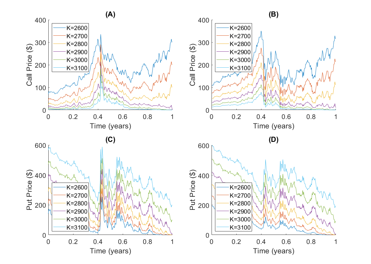
Figure 1 shows the stock price from August 2017 to August 2018 and the corresponding volatility. However, since the BS formula assumes constant volatility, we use the mean volatility (σm = 0.1374) in our simulation. As shown in Figure 2 and Figure 3, the ICN method were found to have very similar solutions and in good agreement with the theoretical results by the Black-Scholes formula. There is no visible difference between the ICN and the RK methods, so the RK figures are not shown here. Both methods cost similar computer resources and give very similar results, and both are in good agreement with the solution obtained by the Black-Scholes formula. For the Black-Scholes formula, we use the built-in function blsprice in the Matlab finance toolbox.

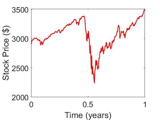
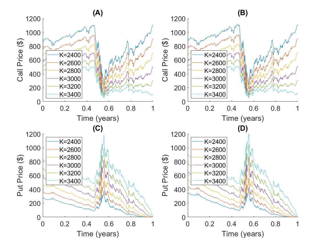
Furthermore, we simulate the S&P500 data from September 2019 to August 2020 when the covid-19 global pandemic occurred. Figure 3 shows the stock price during this period, and we can see the significant drop of stock price when the covid-19 hit the world, where reflected in the middle part of the figure. Figure 4 shows the simulated call and put prices using the ICN method and the B-S formula. There is no visible difference between the ICN and the RK methods, so the RK figures are not shown here.
In the next test, we quantitatively compare the accuracy of the RK4 and the ICN4 methods for the heat equation (11). Results are summarized in Table 1 and Table 2 when σ2 = 2 and 20. Both methods produce similar accuracy where the ICN4 appears to be slightly more efficient. For example, in Table 1, when Nx = 320 both methods have relative error of 1.01 x 10⁻⁶, while the ICN4 costs 0.0209 seconds which is smaller than the 0.0252 seconds for the RK4 method. Similar results are observed in Table 2. When Nx = 320, both methods have relative error of 7.52 x 10⁻⁸ while the ICN4 consumes about 10% less CPU time.
DISCUSSION.
Our findings on computational efficiency indicate that the ICN4 method requires slightly less CPU time compared to RK4 while maintaining the same level of accuracy. As shown in Table 1 and Table 2, ICN4 consumed about 10% less computational time for similar relative errors, making it a preferable option for large-scale simulations where performance is a crucial factor. The advantage of ICN4 in computational efficiency can be particularly valuable for high-frequency trading algorithms or large portfolio risk assessments, where rapid computation is essential.
| Table 1. Comparison of numerical errors for the RK4 method and the ICN4 method when σ = √2. | ||||
| RK4 | ICN4 | |||
| Nx | Relative Error | CPU time (sec) | Relative Error | CPU time (sec) |
| 40 | 6.02E-04 | 0.0009 | 9.44E-04 | 0.0003 |
| 80 | 4.29E-05 | 0.0011 | 4.12E-05 | 0.0011 |
| 160 | 7.16E-06 | 0.0048 | 7.09E-06 | 0.0044 |
| 320 | 1.01E-06 | 0.0252 | 1.01E-06 | 0.0209 |
| Table 2. Comparison of numerical errors for the RK4 method and the ICN4 method when σ = √20. | ||||
| RK4 | ICN4 | |||
| Nx | Relative Error | CPU time (sec) | Relative Error | CPU time (sec) |
| 40 | 1.94E-05 | 0.0025 | 3.62E-04 | 0.0024 |
| 80 | 3.16E-06 | 0.0095 | 3.15E-06 | 0.0097 |
| 160 | 5.32E-07 | 0.0414 | 5.31E-07 | 0.0418 |
| 320 | 7.52E-08 | 0.2213 | 7.52E-08 | 0.2001 |
Another important observation is that market conditions play a significant role in the accuracy of numerical methods. Our simulation of S&P 500 data from September 2019 to August 2020, which covers the onset of the COVID-19 pandemic, highlights how extreme market events can disrupt typical option pricing patterns. The significant drop in stock prices during this period led to increased volatility, which in turn challenges the assumptions of constant volatility in the Black-Scholes model. While the ICN and RK methods performed well under normal conditions, the limitations of assuming constant volatility become more apparent during periods of financial stress. Future research could involve modifying these numerical methods to incorporate stochastic volatility models to better capture real-world market dynamics.
The results of our simulations reinforce the reliability of numerical approaches in solving the Black-Scholes equation, particularly in cases where the volatility remains constant. The agreement between the ICN and RK methods with the Black-Scholes formula suggests that both methods can be effectively applied in practical financial modeling scenarios. However, despite the success of these numerical methods in matching theoretical predictions, it is important to acknowledge that real-world stock markets exhibit more complex behaviors than those captured by the Black-Scholes model.
Over long-time horizons, such as multiple decades, the Black-Scholes model would likely struggle to maintain accuracy due to structural shifts in financial markets. Market conditions change over time due to factors such as technological advancements, economic policies, and evolving trading behaviors. The model assumes that markets remain frictionless and that prices follow a normal distribution, but market structures change. For example, the rise of algorithmic trading and high-frequency trading in modern markets has significantly altered price movements compared to those observed when Black and Scholes first developed their model in the early 1970s.
One consideration to make with the model moving forward would be to implement machine learning or AI into the process of the model. With the rise of machine learning, there is increasing interest in using deep learning to model option pricing. These models can potentially adapt the model to market frictions, making it more accurate to real life. AI would also be able to adapt to the stochastic volatility of the market. Although some modified models already account for stochastic volatility, an AI would be able to adjust in real time to the markets.
Overall, while the Black-Scholes model remains a foundational tool in finance, its performance over long time horizons and during extreme market conditions is limited. Moving forward, hybrid models that incorporate elements of stochastic volatility, jump processes, and data-driven techniques are likely to provide more accurate pricing in complex market environments.
ACKNOWLEDGMENTS.
We acknowledge partial supports from NSF-award 1955664, NSF-award 2219731, and the NIH/NIBIB Center grant 1UG3EB036465.
REFERENCES.
- Black, F., Scholes, M. The pricing of options and corporate liabilities. J. Polit. Econ. 81, 637–654 (1973).
- Merton, R. C. Theory of rational option pricing. Bell J. Econ. Manag. Sci. 4, 141–183 (1973).
- Hull, J. C. Options, Futures, and Other Derivatives. Prentice Hall, Upper Saddle River, NJ, 1997.
- Sørensen, M., Bibby, B., Skovgaard, I. Diffusion-type models with given marginal distribution and autocorrelation function. Univ. Copenhagen Preprint 2003–5 (2003).
- Müller, U., Dacorogna, M., Pictet, O. Heavy tails in high-frequency financial data. In A Practical Guide to Heavy Tails: Statistical Techniques for Analyzing Heavy-Tailed Distributions (Adler, R., Feldman, R., Taqqu, M., Eds.), Birkhäuser, Boston, MA, 1998, pp. 55–77.
- Tankov, P. Financial Modelling with Jump Processes. Chapman and Hall/CRC, Boca Raton, FL, 2003.
- Sircar, K. R., Papanicolaou, G. General Black-Scholes models accounting for increased market volatility from hedging strategies. Appl. Math. Finance 5, 45–82 (1998).
- Heston, S. A closed-form solution for options with stochastic volatility with applications to bond and currency options. Rev. Financ. Stud. 6, 327–343 (1993).
- Hull, J., White, A. The pricing of options on assets with stochastic volatilities. J. Finance 42, 281–300 (1987).
- Burden, R. L., Faires, J. D., Burden, A. M. Numerical Analysis. Cengage Learning, Boston, MA, 2015.
- Teukolsky, S. A. Stability of the iterated Crank-Nicholson method in numerical relativity. Phys. Rev. D 61, 087501 (2000).
- Tran, Q., Liu, J. Modified iterated Crank-Nicholson method with improved accuracy for advection equations. Numer. Algorithms 95, 1539–1560 (2024).

Posted by buchanle on Tuesday, July 22, 2025 in May 2025.
Tags: Black-Scholes model, Iterated Crank-Nicolson method, Stock option