An Analysis of Ice Sheet – Ice Shelf Mechanics through Finite Element Models
ABSTRACT
Physical characteristics of ice sheets and ice shelves, such as the location of the grounding line and ice thickness, play an important role in ice sheet dynamics. These characteristics influence the mechanical stress within the ice shelf that drives fracture propagation and iceberg calving, which is a concern for future sea level rise. This study created a two-dimensional computational model of an idealized floating ice shelf and verified it with an established analytical model based on the Euler-Bernoulli beam theory. This model incorporates generalized boundary conditions for grounded and floating ice regions and was used to study the link between ice shelf geometry (length of the floating ice shelf and ice thickness) and stress, and the potential fracture location based on the maximum normal stress criterion. Our simulations indicate that the point of maximum stress varies greatly depending on the ice shelf length and thickness, with the behavior of short ice tongues following different trends from the behavior of the longer shelves. This preliminary model provides a first-step towards understanding ice sheet dynamics at the grounding line and creating more accurate projections of future sea level rise.
INTRODUCTION.
Floating ice shelves in the Antarctic and Greenland are fracturing and melting at unprecedented rates due to warmer surface air and ocean waters. This has led to an increase of ice sheet mass loss in the recent two decades and estimates of sea level rise ranging from 20 to 200 centimeters within the next century [1-2]]. This increase in such a short period of time holds grave socio economic and physical consequences for the highly populated coastal cities and deltas found around the world [3]. Understanding the dynamic changes and the hydrological feedbacks between the ice sheets and the oceans in relation to increasing global temperatures could allow us to take better preparations and precautions to minimize the impacts of temperature increase and sea level rise.
To have a better understanding of the ice sheet changes, it is important to study the mechanics of ice shelves in relation to physical characteristics, such as the grounding line and ice thickness. The grounding line is the point on the ice body where the sheet, which is grounded onto the bedrock, becomes a floating ice shelf and is a factor in determining the stress state in the entire ice sheet body [4-5]. Understanding the stress state along the ice sheet-ice shelf system is necessary for estimating crevasse (fracture) locations, and for estimating the mass loss from ice sheets (from iceberg calving) and its contribution to future sea level rise.
Ice sheets are massive and slowly evolving bodies, so it is difficult to monitor and track their flow changes with very high resolution. Additionally, a glacier cannot be brought into a laboratory setting, and the time spent monitoring changes over a number of years simply cannot be afforded. Moreover, ice fracture is related to the mechanical stress, which cannot be monitored or measured directly but can only be estimated using theory. Studying the stresses and grounding line are thus most practically and effectively done through computer simulations and models, which can provide a clearer depiction of the ice sheet and environment by enabling the study of specific ice sheet characteristics. Computational simulations utilize equations that describe the physics (Newtonian mechanics) of the ice sheets. Some ice sheet simulations are done using simple 1D models that describe the changes in ice-sheet/shelf length and geometry [6]. To capture greater accuracy, other simulations take into account the conditions surrounding the ice sheet and use 2D models based on ice material behavior [7]. The 2D simulations are capable of capturing complexities in the ice sheets (e.g. boundary conditions and geometries) and allow for the ice sheet mechanics to be well understood. These models, however, need to first be calibrated and validated with experimental/observational data or numerically verified against benchmark solutions. This ensures their accuracy and establishes their predictive capability.
The mechanisms of ice shelf fracture and iceberg calving, and their relation to surface temperatures and melt water are still poorly understood, so the sea level rise projections for the next century have great uncertainty [8-9]. Because fracture is governed by the stress in the ice, the goal of this preliminary study was to examine the stress distribution in an ice sheet – ice shelf system using a 2D finite element model in relation to its geometry (i.e., height and length) and boundary conditions (i.e., floating or grounded). We currently do not consider hydraulic fracture mechanics that can major influence ice shelf fracture [4]. The computer model was validated with an analytical model and then used for parametric studies to understand the relation between physical attributes and behavior.
METHODS.
Mathematical Model for an Ice Sheet and Ice Shelf.
We developed a mathematical model for an ice shelf-ice sheet system assuming that the behavior of the ice is linear elastic. Ice behavior is observed to be viscoelastic, but considering a short time scale, we can make this assumption and model the ice sheet using linear elastic theory [10].
Geometry and Boundary Conditions.
This simulation considered the domain to be of two regions: one being the floating region, the part of the domain which was floating in sea water, and other being the grounded region, the part which we assumed to be resting on bedrock with zero slip condition (Figure 1). The point separating the two regions was the grounding line. From the grounding line to the grounded edge (far-left edge), the bottom boundary was fixed vertically to simulate the ice sheet being grounded to the bedrock. From the grounding line to the terminus (far-right edge), the bottom boundary had the buoyancy force, and the terminal edge had the water pressure.
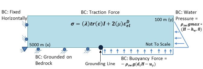
Figure 1. Schematic of a partially grounded ice sheet and floating ice shelf displaying the boundary (the different forces and pressures) and the stress-strain relation in linear elastic theory (shown in the middle of the sheet). In the boundary conditions, 


Governing Equations for the Deformations.
The stress values from the mathematical model and geometries of the ice sheets were input into COMSOL [11] and run using a triangular mesh with a maximum element size of 100m and a minimum element size of 0.625m to see the deformations and stress profile of the ice sheet. This showed the point of maximum stress and hence probable fracturing region. COMSOL was used to model the sheet in 2D using the coefficient form of the partial differential equations module. It was assumed that the ice sheet/ ice shelf was infinitely long in the z-direction and could thus be modeled as a two dimensional plane strain problem. This means that we assumed no strain was experienced in the perpendicular direction to the plane under consideration (Figure 1) and that the displacement in the z-direction was zero. For a plane strain assumption, the linear momentum balance was given through:
\[\frac{\partial\sigma_{xx}}{\partial x}+\frac{\partial\sigma_{xy}}{\partial y}=0\tag{1}\]
\[\frac{\partial\sigma_{xy}}{\partial x} +\frac{\partial\sigma_{yy}}{\partial y} +\rho_{ice}g=0\tag{2}\]
where, 


Validation Studies.
This partially grounded model was validated with a previously developed analytical model proposed by Sayag and Worster [6]. The analytical model was based on the assumption that the response of the ice sheet/ice shelf was one dimensional, so only confined to the horizontal direction. The Euler-Bernoulli beam theory was used to formulate a governing equation for deflection and thus the stresses. Deflection profiles for an ice sheet with a length of 5000m and a grounding line at 2500m from the terminus were obtained from both the analytical model and the 2-D model created in COMSOL to be used for comparison.
Physical Characteristic Analysis.
To compare the physical characteristics of the ice sheet, the dimensions of the partially grounded simulation were manipulated to analyze the relationship between the ice thickness (height), the ice shelf length (floating length), and the size of the calved iceberg. The analysis was done with ice tongue (short ice shelf) lengths of 250m to 500m in increments of 50m and long ice shelf lengths of 1500, 2500, and 3000m. Each of these ice sheets with a different ice shelf length was simulated with heights ranging from 100m to 500m in increments of 100m. For each pair of ice shelf length and height, the x-coordinate along the length where the maximum normal stress occurred and the value of that maximum stress was recorded and then plotted for comparison.
RESULTS.
Comparison to Analytical 1D Model based on Deflection Profiles.
This analysis is conducted to validate the partially grounded computational model. The analytical solution used in this study had already been validated with analogue experimental data in [6], and was thus used to verify our 2D model. The deflection profiles of both the analytical solution and the computational simulation correspond quite closely with a correlation coefficient of r2=0.999 (found using the correlation function in Excel) (Figure 2). The agreement supported the accuracy of the 2D simulation and allowed for further investigation of ice sheet characteristics.
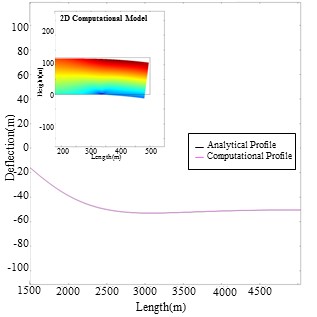
Figure 2. Difference between the deflections profiles of the partially grounded computational model created in this research (shown in the embedded figure of a 2D ice sheet model displaying the deflection and stress profile) and a previously experimentally validated analytical model.
Relation between Ice Sheet Height and the Shelf Length.
The geometry of the ice sheet was found to influence the point of maximum stress and probable fracture. Knowing the relations could aid in creating reliable sea level rise and fracture predictions. The calving length (the distance from the point of maximum stress to the end of the sheet) has been observed to be related to the height [7]. If height were H [7]:
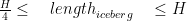
The long ice shelves (longer than 500m) resulted in iceberg sizes that fell within this range. These shelves had displayed a consistent positive, linear trend showing the increase in calving length with increasing height (Figure 3A), which was expected as increasing height leads to increasing weight. The long ice shelves had consistent calving lengths no matter the specific ice shelf length. The ice tongues (ice shelves with a length of 500m or less) broke from this expected, observed range. For most heights, the sheets with the ice tongues followed a parallel trend, though not linear and not always positive. Additionally, unlike the long shelves, the specific calving length varied with each tongue length. The trends occurred starting from a height of 200m, but before then, they were inconsistent. Understanding the cause of the differences in an otherwise regular pattern will require further investigation.

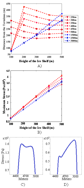
Figure 3. Behavior of a 5000m long ice sheet with thicknesses ranging from 100 to 500m. (A)The length of the calved iceberg for long ice shelves (lengths above 500m, shown in blue) and ice tongues (lengths of 500mand smaller, shown in red). The long ice shelves show a linear positive trend while the ice tongues show inconsistencies up to a height of 200m, but then follow parallel trends. (B)The values of maximum stress for long ice shelves and ice tongues. The two categories of ice shelves display positively increasing trends, with the long shelves increasing linearly and the ice tongues increasing at a rate of change dependent on height. The stress profile is shown of the sheet with a shelf length of 500m and a thickness of (C) 100m or (D) 200m. The ice sheet experiences two peaks in stress, and the maximum peak shifts with increasing height.
The long ice shelves had consistent values of maximum stress, no matter the shelf length that were seen to increase linearly with the increasing height (Figure 3B). The maximum stress values for the ice tongues were also fairly consistent and though not linearly, increased with height. Overall, the long shelves were consistent in calving length and maximum stress values, while the ice tongues had discrepancies for the calving length, but were consistent for the stress values. Although these idealized cases are far from reality, they still describe an interesting behavior with respect to the ice shelves and calving with small floating ice tongues.
The differences in trends between the long ice shelves and the short ice shelves could be caused by the dominant force inducing the bending of the ice sheet. As mentioned in the modeling methods, there were the two main forces from the sea water: the buoyancy force against the bottom and the water pressure against the terminal edge. At longer lengths, the bending that leads to the fracture is largely a result of the ice sheet’s gravitational force [12]. This pushes the ice sheet downwards, eventually increasing the stress to failure of the ice sheet. For the smaller ice sheets, the primary force causing the bending could be the water pressure delivering a compressive force. The different forces could result in different stress values and different locations for the stress to occur.
The variation in location of maximum stress was seen in the stress profile of the ice sheet with a shelf length of 500m. The sheet experienced two peaks of stress. At a height of 100m, the higher peak was closest to the terminus (Figure 3C). With the increase of height to 200m, the maximum peak shifted to that which was closer to the grounding line (Figure 3D). These shifts are seen as the floating length of the ice sheet decreases and could also be attributed to a change in force.
DISCUSSION.
This research presented the process of creating a verified computational model to analyze fracture behavior of ice sheets. The presented model was shown to have deflection profiles similar to that of an established analytical model [6]. This similarity allows for the model to be used in further studies relating the geometry of the ice sheet to the stress profile and fracture behavior.
The simulation created was based on a linear elastic model and made the assumption that the ice was perfectly homogenous. Natural ice tends to have some viscous properties that could result in some deviation from the predicted values given here [5]. Additionally, natural ice can potentially contain imperfections and crevices that could alter the stress profile of the ice sheet. Some ice sheets have been shown to possess multiple points of grounding as the bedrock is not plain and flat [13]. When this occurs, the length of the ice shelf is varied and there can be inconsistencies between the simulated values for the fracture point and the observed values [13]. Computational simulations need to be created to predict the existence of the multiple grounding lines and better understand the fracture behavior and the point of maximum stress when such a circumstance occurs. This simulation involved predicting the fracture point and estimating where the fracture was likely to occur, but the stress profiles produced in the model could be expanded to study the damage mechanics and the initiation and propagation of the fracture.
Having a validated simulation of an ice sheet allows for a better understanding of the mechanics based on the physical characteristics. Simply knowing dimensions of an ice sheet is not very telling, but with a computational simulation, the stresses and the probable point of fracture can be found. From this point, the volume of ice sheet lost can be estimated to show the impact on sea level rise. With this knowledge, people can be better prepared for the potential changes to the environment, some of which are unavoidable at this stage, and encourage the prevention of further temperature increase and sea level rise.
ACKNOWLEDGMENT.
I would like to thank the people that gave their assistance and guidance throughout the duration of this project, including the Vanderbilt Civil Engineering Department, Dr. Lesa Brown and all of SSMV, and Rich Teising for their time and patience. Funding was provided by NSF PLR 1341428.
REFERENCES.
- Alley, R. B. Ice-Sheet and Sea-Level Changes. Science.310, 456–460 (2005)
- National Climate Assessment http://nca2014.globalchange.gov/report/our-changing-climate/sea-level-rise (accessed Jun 3, 2017).
- Nicholls, R. J.; Cazenave, A. Sea-Level Rise and Its Impact on Coastal Zones. Science. 328, 1517–1520 (2010)
- Pollard, D.; Deconto, R. M.; Alley, R. B. Potential Antarctic Ice Sheet retreat driven by hydrofracturing and ice cliff failure. Earth and Planetary Science Letters. 412, 112–121 (2015)
- Rignot, E. Rapid Bottom Melting Widespread near Antarctic Ice Sheet Grounding Lines. Science. 296, 2020–2023 (2002)
- Sayag, R.; Worster, M. G. Elastic response of a grounded ice sheet coupled to a floating ice shelf. Physical Review E. 8, (2011)
- Christmann, J.; Plate, C.; Müller, R.; Humbert, A. Viscous and viscoelastic stress states at the calving front of Antarctic ice shelves. Annals of Glaciology. 57, 10–18 (2016)
- Deconto, R. M.; Pollard, D. Contribution of Antarctica to past and future sea-level rise. Nature. 531, 591–597 (2016)
- Ritz, C.; Edwards, T. L.; Durand, G.; Payne, A. J.; Peyaud, V.; Hindmarsh, R. C. A. Potential sea-level rise from Antarctic ice-sheet instability constrained by observations. Nature. 531, 115-118 (2015)
- Stephens, R. The mechanical properties of ice. II. The elastic constants and mechanical relaxation of single crystal ice. Advances in Physics.7, 266–275 (1958)
- COMSOL Multiphysics® and COMSOL Server™ Version 5.3a https://www.comsol.com/ (accessed Jun 3, 2017).
- Scambos, T.; Fricker, H. A.; Liu, C.-C.; Bohlander, J.; Fastook, J.; Sargent, A.; Massom, R.; Wu, A.-M. Ice shelf disintegration by plate bending and hydro-fracture: Satellite observations and model results of the 2008 Wilkins ice shelf break-ups. Earth and Planetary Science Letters.280, 51–60 (2009)
- Dawson, G. J.; Bamber, J. L. Antarctic Grounding Line Mapping From CryoSat‐2 Radar Altimetry. Geophysical Research Letters. 44, 11,886–11,893 (2017)
Posted by John Lee on Tuesday, December 22, 2020 in May 2018.
Tags: Finite element model, Fracture, Ice sheet, Mechanical stress