Quadrotor PID Control Made Easy

ABSTRACT

This paper aims to facilitate the understanding of Position-Integral-Derivative (PID) controllers and their roles in quadrotors. However, there are difficulties in understanding quadrotor dynamics due to the usage of differential equations and the existence of 6 degrees of freedom in quadrotor movement. Easy visualization of quadrotor dynamics is made possible by a hands-on simulation from Github, which eliminates the need to go into differential equations. The input of the quadrotor consists of four values which are then transformed to the needed individual motor speeds by a series of calculations. The PID controller controls these four values by getting feedback from errors, which are the distances from the target location. Many studies have compared PID controllers with other types of controllers including efficiency and stability. These studies often lack clear explanations on how to tune the KP, KI, and KD values. Using a quadrotor PID control simulation, this paper takes a trial-and-error approach to better understand the effects of PID control parameter settings and establishes specific steps to tune a PID controller.

INTRODUCTION.

Quadrotors have 4 rotors and 6 degrees of freedom (1). They utilize thrust and torque on different axes in order to move. Their rotor blades rotate in opposite directions to counterbalance the torque generated by the motors. The configuration of the 4 motors refers to the ability of the quadrotor to move accurately and precisely according to the inputs provided (1) and is critical for stable and controlled flight. When a quadrotor tilts, the forces are then split along the x, y, and z-axis to provide an understanding of the forces acting on the quadrotor (1). However, a set of three differential equations is required to represent the movement of quadrotors (1), which makes it difficult for most people to understand.

The differential equations are derived from Newton’s second law, where \(force = mass * acceleration\ \)(4). These differential equations are represented using 3×3 matrices (1) to help model the influence of estimated external forces and torques on the quadrotor’s behavior. Quadrotor simulators based on these models are available on GitHub (5).

Quadrotors typically use one of two types of controllers: a Position-Integral-Derivative (PID) or a Linear-Quadratic Regulator (LQR). LQRs are more robust, but PIDs have better responses to input (2). Here, we focus on PID controllers, which have been implemented into quadrotors controlling their movement based on their physics model, which are equations that can predict how the quadrotor reacts to different input from the four motors (2) and have been utilized for automatic height control for the drones when doing tea-farm inspection (3).

A PID controller gets the input from the errors and then calculates the derivative and integral of the errors (1). The KI, KP, and KD are all constants. The KI value is multiplied with the integral of the error between the desired quadrotor state and the current quadrotor states (5). The KP is multiplied with the value of the error (5). The KD is multiplied with the derivative of the error (5). The resulting values are then added together as inputs to U1, U2, U3, and U4, which control throttle, yaw, roll, and pitch (5).

Most of the papers focus on implementing a PID controller and calculating the PID values using the Ziegler-Nichols method (2). The Ziegler-Nichols method sets the KI and KD are set to zero, then increase the KP until the system oscillates; the KI and KD values are calculated with a set relationship with the KP value; this leads to the optimized values for the function (2). However, none include instructions about how to tune a PID controller set for the KI, KP, and KD value without an alternate method that does not involve starting the tuning process by setting all values to zero. The main disadvantage is that the Ziegler-Nichols method involves oscillations that may be risky when tuning a quadrotor and may need lots of time to achieve the oscillations wanted. Also, using a simulation will make visualization of the PID tuning more intuitive without needing differential equations. Therefore, there is a need to find another way to tune PID values.

MATERIALS AND METHODS.

Obtaining the Simulation.

The Matlab QuadSimAP simulation shows the effect of different inputs on the behavior of the quadrotor (5). This allows an easier understanding of the dynamic model of the quadrotor. The simulation also helps with understanding PID values and their impact on the behavior of the quadrotor. Fig. 1 shows how the quadrotor is defined and how the four motors are located relative to quadrotors. The axes for the quadrotor are also shown, which will aid the explanation later.

Using a Trial-and-error Method.

I derived my own tuning method for a PID controller with already given values.

1. If there is an overshoot, then decrease the KP and KI value by 90 percent at a time.
2. Repeat this until it reaches the desired altitude stably.
3. Increase the KP by 10 percent until it reaches a desirable speed.
4. increase or decrease the KD by 10 percent depending on the overshoot.

Increasing the KP and KI will make the quadrotor have higher acceleration, but it will increase the overshoot of the quadrotor. The KI term is used for steady state error, so if the quadrotor is constantly having a positive difference between the achieved altitude and desired altitude, decreasing the KI will let the quadrotor settle to the correct height. After the height is correct, there is no need to increase the KI as KI will contribute to a wrong final height. Instead, increasing the KP will ensure the height is correct while the speed of the quadrotor is increased. The KD term will decrease the overshoot of the quadrotor.

RESULTS.

Experiment 1 – Testing the Z-Axis Altitude Control.

The targeted height was set to 6m for the PID controller while sensor errors were disabled in the simulation. Additionally, during the experiment, Z-axis quadrotor dynamics derived by Yun Li and Yuntang Li (1) were substituted in the quadrotor simulation.

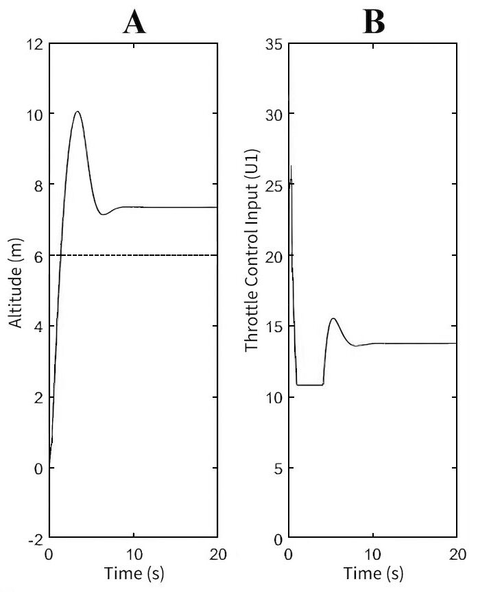
The original PID values shown in Table 1 result in the quadrotor overshooting the desired amplitude of 6m by 1.2m (Fig. 2A). The large overshoot shows that the KP and KI values of the quadrotor are too high, so the values are lowered. The lower throttle input in the second half Fig. 2B show that the throttle is trying to control the height of the quadrotor. However, the quadrotor ended at the incorrect height, showing that the PID controller’s KI value has not been adjusted enough to eliminate steady-state errors.

Table 1. Variables set when the data in Fig. 2 & Fig. 3 were obtained in the experiment
Both	Figure 2	Figure 3
Thrust: 40 N Simulation time: 20 seconds Sampling time: 0.01 seconds	Quad.Z_KP=5.8 Quad.Z_KI=50 Quad.Z_KD=-5.05	Quad.Z_KP=79 Quad.Z_KI=20 Quad.Z_KD= -130

In contrast, Fig. 3 shows the behavior of the quadrotor after retuning the PID values using the aforementioned method. The smooth curve in Fig. 3A shows the reduction in the overshoot. Interestingly, the controller’s output proved more accurate than the values initially provided by William Selby. This observation highlights the dynamic nature of PID values, which adapt based on the desired state of the object.

According to Table 1, one can see the different values for the KP, KI, and KD values for the quadrotor. In the scenario of Fig. 3, the KP value multiplies the error by 79 and adds to the input of the quadrotor, while the 20 value of KI means the integral of the errors are multiplied by 20. The –130 value for KD shows that the derivative of the error is multiplied by these values. These three values are then added together to provide the input of U1 which is drawn in Fig. 3B.

Experiment 2 – Testing the X- and Y-Axis Controls.

The value of the targeted height of the quadrotor is changed to 2 meters for vertical movement in the Z axis. The X and Y axis PID controller testing is achieved by changing the desired X and Y coordinates to 1 m both.

The PID values shown in Table 2 reflect the difference in the movement of the quadrotor between Fig. 4 and Fig. 5. Fig. 4A and Fig. 4B shows the quadrotor having increasing oscillations along the X and Y axis. This shows that the KP and KI values are both too large for the PID controller for the quadrotor. After using the trial-and-error method, and simulating with reduced KP, KI, and KD values, stability was restored. The quadrotor now has a more stable approach to the desired location (Fig. 5).  Using Fig. 1, we can see that the quadrotor rolls and pitches at the same time in order to move on both the X and Y axes. The quadrotor does not have yaw as it is still facing the same direction.

Table 2. Variables set when the data in Fig. 4 & Fig. 5 were obtained in the experiment
Both	Figure 4	Figure 5
Thrust: 40 N Simulation time: 10 seconds Sampling time: 0.01 seconds	Quad.X_KP = 0.35 Quad.X_KI = 0.25 Quad.X_KD = -0.35 Quad.Y_KP = 0.35 Quad.Y_KI = 0.25 Quad.Y_KD = -0.35 Quad.Z_KP = 5.8 Quad.Z_KI = 0 Quad.Z_KD = -5.05	Quad.X_KP = 0.2 Quad.X_KI = 0 Quad.X_KD = -0.3 Quad.Y_KP = 0.2 Quad.Y_KI = 0 Quad.Y_KD = -0.3 Quad.Z_KP = 15 Quad.Z_KI = 0 Quad.Z_KD = -15

 

 

DISCUSSION.

In the simulation, one can see the effects of the PID values on the controller. A meticulously tuned PID controller can have a significant effect on the behavior of the quadrotor, enabling better stability and precise control, particularly when moving longer distances from a starting point. The importance of tuning these parameters becomes evident as poorly chosen values lead to oscillations, instability, or delays in reaching the desired state. Future improvements to the experiment include using a real-life quadrotor, as some errors inherent to physical systems, such as inaccuracies in GPS readings, altimeter data, and external disturbances like wind, cannot be replicated fully in a simulated environment. Additionally, potential discrepancies in simulated forces, where thrust production is considered ideal, may cause the results to differ from real-world behavior.

Visualization can further enhance the understanding of PID tuning. For example, a graph plotting the relative PID values against the desired state of the quadrotor would provide clearer insights into how the proportional, integral, and derivative terms impact its performance. Testing in real-life scenarios would also allow for a more accurate evaluation of how environmental errors, input signal delays, and unmodeled dynamics influence the behavior of the quadrotor. These tests could reveal whether adjustments to PID values are needed to account for such factors.

CONCLUSION.

It has been observed that achieving the desired state for a quadrotor using a PID controller requires careful tuning of the proportional, integral, and derivative values. These PID parameters are not universally fixed and must be tailored to the specific dynamic requirements of the system. Using a pre-tuned PID controller for a predetermined state, rather than beginning from zero, significantly accelerates the tuning process and enhances efficiency. The trial-and-error approach further refines this process, allowing the quadrotor to achieve stable control faster.

ACKNOWLEDGMENTS.

I would like to thank Professor Shi-Chung Chang from Department of Electrical Engineering of National Taiwan University for his inspiration, invaluable guidance, and mentorship throughout this research. I would like to thank Professor Ruey-Beei Wu for providing me with the opportunity to work with the NTU UAV Research Team. I would also like to extend my gratitude to the students at the Control & Decision Laboratory and the Wireless IoT Laboratory at National Taiwan University for their exceptional technical knowledge and support. This work was supported in part by the National Science and Technology Council, Taiwan, R.O.C., under grant NSTC 113-2218-E-002-049.

REFERENCES

1. J. Li, Y, Li, “Dynamic analysis and PID control for a quadrotor” in 2011 IEEE International Conference on Mechatronics and Automation (IEEE, 2011), pp. 573-578.
2. D. Khatoon, D. Gupta, L. K. Das, “PID & LQR control for a quadrotor: Modeling and simulation” in 2014 International Conference on Advances in Computing, Communications, and Informatics (IEEE, 2014), pp. 796-802.
3. A. T. L. Chua, “Research on relative height control and Wi-Fi-6 integrated in-band communication of drones for tea farm inspection,” thesis, National Taiwan University, Taipei, (2022).
4. C. D. McKinnon, A. P. Schoellig, Estimating and reacting to forces and torques resulting from common aerodynamic disturbances acting on quadrotors. Robot. Auton. Syst. 123, C (2020).
5. W. Selby, MatlabQuadSimAP, version 1, Github (2015); https://github.com/wilselby/MatlabQuadSimAP.

---

---

Posted by buchanle on Thursday, July 3, 2025 in May 2025.

Tags: Dynamics, PID Control, Quadrotor