Automating Human Sleep Staging Analysis from Polsomnographic Recordings with a Discrete Hidden Markov Predictive Model

ABSTRACT

The identification of sleep stages is a necessary step in any sleep study. Previous attempts to conduct this identification using manual methods were tedious and inefficient. More recent methods have come to rely on automatic identification conducted through several different means. One of these is Hidden Markov Model (HMM) based sleep staging. This method was a definite improvement, but the accuracy of the results was still poor, possibly because the transition conditions were not included in the HMM modeling process. In sleep staging, the sleep stage transition highly depends on the current stage. In this paper, transition probabilities were incorporated into the HMM leading to an improvement in the accuracy of the model. This project proposes an automatic sleep stage scoring approach from polysomnographic recordings with a Discrete Hidden Markov Predictive Model (DHMM). The Polysomnographic (PSG) dataset from PhysioNet Sleep EDF-Database was used which contained whole-night polysomnographic sleep recordings containing electroencephalographic (EEG), electrooculographic (EOG), chin electromyographic (EMG), and event markers. Eighty percent of the data was used for training the DHMM, and the remaining twenty percent of the data was tested by the trained DHMM. The features were extracted from the frequency-domain (spectral) representation of the EEG, EOG, and EMG signals by signal transformation from time domain to frequency domain. The primary metric for measuring the model success was accuracy. Compared with the gold standard of manual scoring using Rechtschaffen and Kales criterion, the overall average accuracy applied on 50 PSG records reached 80.20%, proving that it is a promising start in the venture to automate sleep analysis for the future.

INTRODUCTION.

50-70 million Americans suffer from sleep or wakefulness disorders. Since patients experience symptoms during sleep, they are not easily detectable, and therefore most sleep disorders remain undiagnosed. Sleep deficiency and anomalies in sleep architecture are linked to many chronic health problems, including sleep apnea, diabetes, stroke, brain injury, Parkinson’s disease, depression, and Alzheimer’s disease. Diagnosing sleep disorders leads to the early detection of other health conditions [1]. Patterns in sleep architecture can be used for reliable clinical diagnosis on individuals as well as to track disease progression over time. Clinical sleep diagnosis requires a polysomnography (PSG) study to measure overnight electroencephalogram (EEG), electrooculogram (EOG), electrocardiogram (ECG), airflow, and other signals. After data is collected, an expert currently must spend up to 2 hours to score and manually annotate the sleep stages observed throughout the night by following the Rechtschaffen & Kales (R&K) rules presented in 1968. Therefore, PSG studies are expensive and often only used after significant progression of a patient’s symptoms. Each epoch (i.e. 30 s of data) is classified into one of the sleep stages including wakefulness (Wake), non-rapid eye movement (stages 1–4, from light to deep sleep) and rapid eye movement (REM). Recently, stages 3 and 4 were combined and are now known as the slow wave sleep stage (SWS) or deep sleep [2]. Manually scoring on PSG data by experts is labor intensive. Therefore, sleep automatic sleep stage scoring approaches have been developed. They include a knowledge-based approach to sleep EEG analysis [3], time domain analysis [4], [5], Artificial Neural Network [6], [7] and HMMs [8-10].

HMMs are a class of probabilistic graphical models that enable the prediction of a sequence of unknown (hidden) variables from a set of observed variables. HMMs are sequence models in which a discrete stochastic process moves through a series of states that are ‘hidden’ from the observer. In an HMM, the result of the previous state influences the result of the next state. Therefore, an HMM is ideal for sleep based on the principle that the result of one stage influences the result of the next stage and was selected for the study.

HMM-based sleep staging has been researched during previous studies; however, the sleep stage transition probabilities were not included in the HMM [8-10]. In this work using the HMM sleep model, the transition probabilities in the HMM were considered. This resulted in improvements in the accuracy of the HMM and thus the accuracy of sleep staging. The proposed DHMM allows Sleep Staging Analysis to be automated, making it more efficient and cost effective.

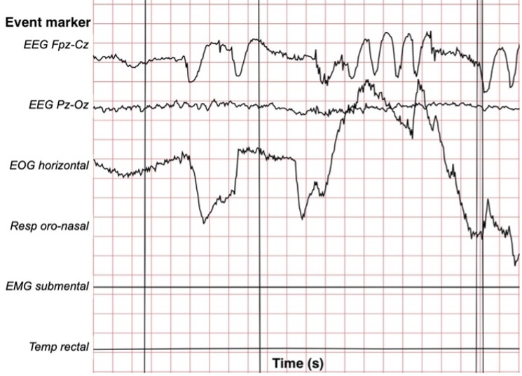
Figure 1. Visualization of EEG waveform with EEG Fpz-Cz, EEG Pz-Oz, EOG horizontal, Resp oro-nasal, EMG submental, and Temp rectal event markers.

MATERIALS AND METHODS.

Polysomnography. Polysomnography is another term for a sleep study and is a comprehensive test used to diagnose sleep disorders. Polysomnography records one’s brain waves (EEG), blood oxygen level, heart rate (ECG) and breathing, as well as eye (EOG) and leg movements (EMG). A PSG dataset from PhysioNet was acquired, [11] which contains whole-night polysomnographic sleep recordings containing EEG, EOG, chin EMG, and event markers. In the dataset recordings were obtained from 83 Caucasian males and females (21–101 years old) without any medication. The data contains horizontal EOG, Fpz-Cz and Pz-Oz EEG, each sampled at 100 Hz. The sc* recordings also contain the submental-EMG envelope, oro-nasal airflow, rectal body temperature and an event marker, all sampled at 1 Hz. The st* recordings contain submental EMG sampled at 100 Hz and an event marker sampled at 1 Hz.

Hypnograms were manually scored according to the R&K rules based on Fpz-Cz / Pz-Oz EEG instead of C4-A1 / C3-A2 EEGs. Figure 1 depicts what each PSG file looks like.

Pre-processing of Data. In this stage of data processing, annotations which had long sequences of the awake stage were removed from the beginning and the end. Epochs, or specific time-windows, were extracted from the continuous EEG signal. The duration of fixed length epochs of 30 seconds was selected in order to achieve better frequency resolution in the frequency domain.

Feature Extraction from EEG Signal. The features from the EEG signal of each sleep stage were extracted in the frequency domain. 6 features in the frequency domain were used. The different brain waves, namely delta, theta, alpha, and beta reside in specific frequency ranges. First, a Fast Fourier Transform (FFT) was applied to the epochs. Following the FFT, the power spectrum was calculated for the sleep stage for the band 0-30 Hz for the EEG, EOG and EMG, also referred to as the total power. The mean of the total power was then computed along with the delta, theta, alpha, and beta band power ratios.

DHMM for Sleep Staging. In this step, codebook generation and vector quantization were performed for sleep stage classification. In the DHMM, the transition probabilities or state transition matrix is used to improve the accuracy of the model and sleep staging. The next sleep stage is also highly dependent on the current stage, which means that the probability of a sleep stage transition is dependent on the current sleep stage as well.

Vector Quantization and Codebook Generation. Vector quantization is a technique to quantize signal vectors in order to determine the center points that best represent the data by partitioning it into regions. The mean of the points within each region is then taken which becomes its new center point. With each iteration, the center points become more characteristic of all the points. This is repeated until the center points stabilize. The feature vectors are real number vectors in real space with 6 dimensions. Vector quantization of these feature vectors is necessary in order to reduce the computational overhead. Following the steps outlined above, a codebook was created during the step of feature vector quantization so that the result of the vector quantization was a set of observation or epoch codes for the DHMM implementation. 20 feature groups were selected and center points from the data from which the regions were designed. This process returned the code book and epoch codes, or observation codes used in DHMM.

DHMM and Sleep Stages. In DHMM the outputs of each state are observed, rather than the states themselves. There is a probability distribution for each state over the possible output. The sequence of outputs generated by the DHMM thus provides data regarding the sequence of hidden states. The following algorithm was adapted from [12].

The 5 parameters to DHMM were

\(\lambda\): DHMM, \(\lambda =\left\{A, B, \pi, N, M\right\}\)

A: transition probability or state transition matrix

B: observation or emission probabilities or probability distribution when at a given state

\(\pi\): initial state distribution

N: number of possible states

M: number of observations

\(O={O_1,O_2,O_3,\ldots O_T}\) where the \(O_i\) element is part of the vocabulary of observations with M elements.

In sleep staging the states which are hidden behind the DHMM can be estimated by observation which is measured for each of the states in the DHMM. The DHMM was built using the Viterbi Algorithm. This algorithm determines what sequence of states most accurately describes the sequence of observations, where O₁, O₂, O₃, … Oₜ are the observations and q₁, q₂, q₃, … qₜ are the states as below

\[O={O_1,O_2,O_3,\ldots O_T}\tag{1}\]

\[Q={q_1,q_2,q_3,\ldots q_T}\tag{2}\]

In this approach, the sequence of states is the sleep data which is passed as an input to the model and the number of observations was 20. Therefore, one way of solving for the best fit can be completed by choosing states that are individually most likely at a time t given the observation O and the \(\lambda\). This leverages as below:

\[\gamma_t\left(i\right)=P\left(q_t=S_i\middle|\ O,\lambda\right)\tag{3}\]

In Eq. 3, \(\gamma_t\) is a probability that one is in state i at a time \(q_t\) with the observation O and the \(\lambda\).

Eq. 3 can be answered using \(\alpha\) and \(\beta\) components as below:

\[\gamma_t\left(i\right)=\frac{\alpha_t\left(i\right)\beta_t\left(i\right)}{P\left(O/\lambda\right)}=\frac{\alpha_t\left(i\right)\beta_t\left(i\right)}{\sum_{j=1}^{N}{\alpha_t\left(j\right)\beta_t\left(j\right)}}\tag{4}\]

\[\sum_{i=1}^{N}{\gamma_t\left(i\right)}=1\tag{5}\]

Eq. 5 of \(\gamma\) therefore ensures that \(\gamma_t(i)\) is thus a probability and \(\alpha_t(i)\) is the probability that regardless of the path, it ends up in state i at time t, after seeing all the observations up until time t. The \(\alpha\) term is called the forward term.

\(\beta_t(i)\) is the probability that starting in state i one would see all the remainder of the observations up until time T. The \(\beta\) term is the backward term. They together form the basis of the Forward-Backward algorithm. States 1 through N are the states that the model goes through.

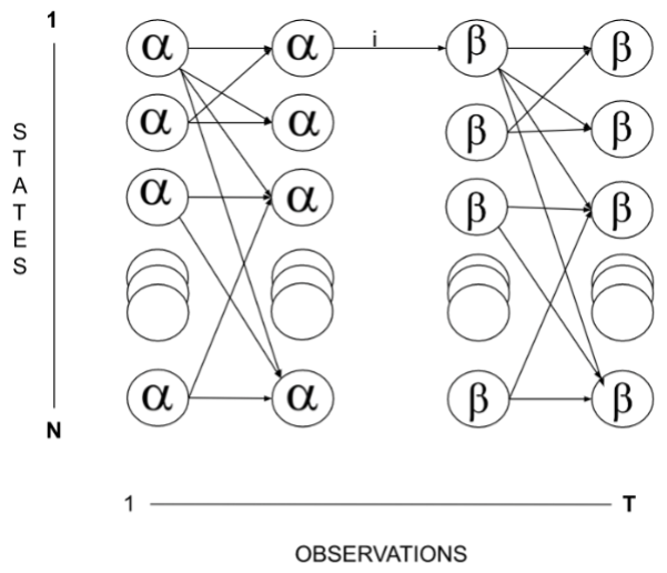
Figure 2. Lattice diagram depicting alpha and beta terms spanning states 1 to N over a time period of observation 1 to T.

In Eq. 4, the numerator \(\alpha\) and \(\beta\) can be calculated efficiently and the sum in the denominator can also be calculated. Thus, by combining \(\alpha_t(i)\) and \(\beta_t(i)\) it is ensured that the sum over all states of \(\gamma_t(i) = 1\) or \(\gamma_t(i)\) is thus a probability and visually looks as in the lattice diagram (Fig. 2). This helps discern the probability of being in state i at a moment of time to the final time T. Also, by joining \(\alpha_t(i)\) and \(\beta_t(i)\) the probability of getting to a state and leaving from the state is obtained.

\[q_t={argmax}_{1\le i\le N}{\gamma_t\left(i\right)},\ 1\le t\le T\tag{6}\]

This helps solve for \(\gamma_t(i)\). The expected number of correct states is maximized; however, the result may not make sense as DHMM is a dependent model which handles sequential data.

There is a second way of solving for the best fit by choosing a path sequence that maximizes a complete sequence of states that are possible given the observations and the model.

P(Q|O,\(\lambda\)) where P is the Probability, Q is the sequence of states, O is the sequence of observations, and \(\lambda\) is the model.

This is equivalent to maximizing the state sequence and the observation sequence in a coherent pattern with the given model as given below.

\[P\left(\{q_1,q_2,\ \cdots\ q_T\},\{O_1,O_2,\cdots\ ,O_T\}\middle|\lambda\right)\]

This is solved by Viterbi’s algorithm as below

\[\delta_t\left(i\right)=\max_{q_1,q_2,\cdots q_{t-1}}{P}\left(\{q_1,q_2,q_3,q_t=i\},\{O_1,O_2,O_3,O_t\}\middle|\lambda\right)\tag{7}\]

Eq. 7 comes down to the best sequence of states that maximizes the probability of seeing the states and observations, given the model itself.

The above is solved using Induction. The basic inductive step is defined as below:

\[\delta_{t+1}\left(j\right)=\left[\max_ i{\delta_t\left(i\right)a_{ij}}\right]\cdot b_j\left(O_{t+1}\right)\tag{8}\]

Eq. 8 helps with getting the state that maximized \(\delta\) at a previous time step i , and then helped in getting from state i to state j. In this one, therefore, there is a need to keep track of where one comes from and the value of i which maximizes the result at each of time step so that the path can be recreated. In order to keep track of this, a new variable is required which records the state that one came from.

Initialization Step. In the first time-step, Viterbi initializes \(\delta_1(i)\) as the probability of starting in state i. Observing the first observation and \(\psi_1\left(i\right)\) helps in getting which state the path came from, given the current state. This is initialized to 0 since this is the start of the path.

\[\delta_1\left(i\right)=\pi_ib_i\left(O_1\right),{\ \psi}_1\left(i\right)=0\tag{9}\]

Inductive Step. The inductive step helps with getting the probability of the best sequence of states that gets to state j consisting of an achievable sequence of states. The states that the path can come from are 1 to N.

\[\delta_t\left(j\right)=\max_{1\le i\le N}{\left[\delta_{t-1}\left(j\right)a_{ij}\right]}\cdot b_j\left(O_t\right)\tag{10}\]

\[\psi_t\left(j\right)={\rm argmax}_{1\le i\le N}{\left[\delta_{t-1}\left(j\right)a_{ij}\right]}\tag{11}\]

Termination Step. The termination step is defined by a valid sequence of states and is the sequence of state that has the highest \(\delta_T(i)\) at the final time step. The state that the model will be in is the state for the corresponding \(\delta\). If it is needed to figure out recursively which state the path came from, the \(\psi\) variable can be used to track the way back.

\[P^\ast=\max_{1\le i\le N}{\delta_T\left(i\right)}\tag{12}\]

\[q_T^\ast=arg{max}_{1\le i\le N}{\left[\delta_T\left(i\right)\right]}\tag{13}\]

\[q_t^\ast=\psi_{t+1}\left(q_{t+1}\right)\tag{14}\]

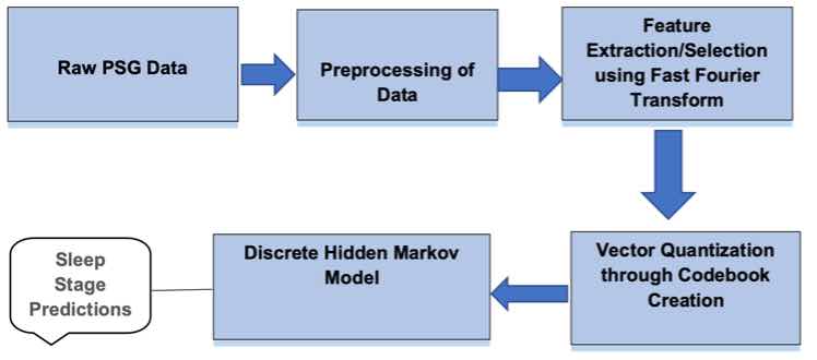
Figure 3. Design Flow Diagram showing the steps from raw PSG data to sleep stage predictions using the DHMM.

Sleep Staging Procedure. First, the sleep annotations or Hypnogram.edf file was read. This sleep annotations file contained the annotations of the sleep patterns that correspond to the PSG. Next, the sleep stages read from the annotations file were preprocessed to remove the long sequences of the awake state at the beginning and the end. Afterwards, the sleep data or PSG.edf file was read which contained whole-night polysomnographic sleep recordings. Then, the epochs from the PSG.edf files were loaded by selecting an epoch length of 30 seconds and sampling frequency of 100Hz. Following this, the features in the frequency domain were extracted by taking the loaded epochs in the previous step as an input. After, these features were converted to a codebook by taking the features extracted in the previous step. The output of this process was the epoch codes. Subsequently, the output of epoch codes was split into test and training sets by using a training percentage of 0.8. The sleep annotations or sleep stages were also split into test and training sets by using a training percentage of 0.8. Next, a DHMM was created by passing the finite states from the sleep EDF annotations file and finite number of observations. The DHMM was trained by taking the training sleep data and the epoch codes training data. After, the Viterbi algorithm was executed to calculate the hidden states by taking the epoch codes test data as an input. Then, the sleep stages were predicted using the sleep staging model. Finally, the accuracy of the model was calculated by comparing the actual sleep stages against the predicted sleep stages. Figure 3 illustrates the sleep staging procedure.

RESULTS.

The above sleep model described in the sleep staging procedure was tested against 50 records. The overall average accuracy was 80.20% against the 50 PSG records the model was tested on. The top 10 records are shown in Table 1.

Table 1. Accuracy of Top 10 records including annotations and data files.
Annotations File	Data File	Accuracy (%)
SC4011EH-Hypnogram.edf	SC4011E0-PSG.edf	93.4
SC4081EC-Hypnogram.edf	SC4081E0-PSG.edf	89.7
SC4082EC-Hypnogram.edf	SC4082E0-PSG.edf	87.2
SC4171EU-Hypnogram.edf	SC4171E0-PSG.edf	89.3
SC4432EM-Hypnogram.edf	SC4432E0-PSG.edf	94.0
SC4482FJ-Hypnogram.edf	SC4482F0-PSG.edf	93.0
SC4651EP-Hypnogram.edf	SC4651E0-PSG.edf	97.2
SC4662EJ-Hypnogram.edf	SC4662E0-PSG.edf	98.1
SC4002EC-Hypnogram.edf	SC4002E0-PSG.edf	86.6
SC4601EC-Hypnogram.edf	SC4601E0-PSG.edf	87.8

The model was most effective at predicting Sleep Stage 3 (Slow wave sleep or deep sleep) and Sleep Stage 4 (Rapid-eye movement sleep). However, it was least effective at predicting Sleep Stage 1 (the transition period between wake and sleep). This is hypothesized to be due to humans spending far less time in Sleep Stage 1 (<10 mins) as compared to Sleep Stages 3 (20 – 40 mins) and 4 (10 – 60 mins) [13]. As a result, there are fewer annotations for Sleep Stage 1 and the model is not trained as thoroughly as it is for the other sleep stages.

DISCUSSION.

In this paper, an automatic human sleep staging analysis from polysomnographic recordings with a Discrete Hidden Markov Predictive Model was proposed. 6 features were selected for the work and the model developed helped in classifying sleep stages with great accuracy. The model was most effective at predicting Sleep Stage 3 (Slow wave sleep or deep sleep) and Sleep Stage 4 (Rapid-eye movement sleep), and it was least effective at predicting Sleep Stage 1 (the transition period between wake and sleep).

Although previous work in Sleep Stage Identification has used HMM based sleep staging, the transition conditions were not included in the HMM. Including the transition conditions improved the accuracy of the model. The overall average accuracy applied on 50 PSG records reached 80.20%.

In the future, the accuracy can be measured for each individual sleep stage by enhancing the algorithm. The difficulty of making predictions for sleep stage 1 can be addressed by training the model to recognize the high amplitude theta waves that it is characterized by. The results prove the viability of automation of Sleep Staging Analysis. Sleep Analysis is important in diagnosing conditions like hypersomnia, insomnia, narcolepsy, obstructive sleep apnea (OSA) and periodic limb movement disorder (PLMD). The automation of sleep analysis is meaningful in the reduction of human involvement and as a result the cost associated for such analysis. This would help improve the quality of life for patients as well as the early detection of many diseases. The model can be easily applied to aspects of EEG analysis other than sleep such as identifying seizures and epilepsy, leaving direction for this research to expand in the future.

ACKNOWLEDGMENTS.

Thank you to Ms. Sushma Bana for being my mentor for this project.

REFERENCES

H. R. Colten, B. M. Altevogt. Sleep Disorders and Sleep Deprivation: An Unmet Public Health Problem. The National Academies Press. 1, 55-56 (2006).
2. A. V. Esbroeck, B. Westover. Data-Driven Modeling of Sleep Staging from EEG. Annual International Conference of the IEEE Engineering in Medicine and Biology Society. 3, 50-55 (2012).
3. B. H. Jansen, B. M. Dawant. Knowledge-based approach to sleep EEG analysis– a feasibility study. IEEE Transactions on Biomedical Engineering. 36, 510–518 (1989).
R. Maulsby, J. Frost, M. Graham. A simple electronic method for graphing EEG sleep patterns. Electroencephalography and Clinical Neurophysiology. 21, 501–503 (1966).
H. W. Agnew, J. C. Parker, W. B. Webb, and R. L. Williams. Amplitude measurement of the sleep electroencephalogram. Electroencephalography and Clinical Neurophysiology. 22, 84-86 (1967).
H. Park, K. Park, D. Jeong. Hybrid neural-network and rule-based expert system for automatic sleep stage scoring. Proceedings of the 22nd Annual International Conference of the IEEE Engineering in Medicine and Biology Society. 2, 13-17 (2000).
F. Ebrahimi, M. Mikaeili, E. Estrada, H. Nazeran. Automatic sleep stage classification based on EEG signals by using neural networks and wavelet packet coefficients. 2008 30th Annual International Conference of the IEEE Engineering in Medicine and Biology Society. 5, 1151-1154 (2008).
L. G. Doroshenkov, V. A. Konyshev, S. V. Selishchev. Classification of Human Sleep Stages Based on EEG Processing Using Hidden Markov Models. Biomedical Engingeering. 41, 25–28 (2007).
A. Flexer, G. Dorffner, P. Sykacekand, I. Rezek. An Automatic, Continuous and Probabilistic Sleep Stager Based on A Hidden Markov Model. Applied Artificial Intelligence. 16, 199-207 (2002).
A. Flexer, G. Gruber, G. Dorffner. A reliable probabilistic sleep stager based on a single EEG signal. Artificial Intelligence in Medicine. 33, 199–207 (2005).
B. Kemp, A. H. Zwinderman, B. Tuk, H. A. C. Kamphuisen, J. J. L. Oberyé. Sleep-EDF Database. Analysis of a sleep-dependent neuronal feedback loop: the slow-wave microcontinuity of the EEG. IEEE Transactions on Biomedical Engineering. 47, 1185-1194 (2000).
D. J. Patterson. Hidden Markov Models. Youtube.com/@djp3. < https://www.youtube.com/playlist?list=PLix7MmR3doRo3NGNzrq48FItR3TDyuLCo> (2020).
E. Suni, N. Vyas. Stages of Sleep: What happens in a Sleep Cycle | Sleep Foundation. <https://www.sleepfoundation.org/stages-of-sleep> (2022).

Posted by John Lee on Tuesday, May 30, 2023 in May 2023.

Tags: Hidden Markov model, polysomnography., sleep staging analysis