Evaluation of Food Insecurity Risk Through Principal Component Analysis: A Case Study in Travis County, Central Texas

ABSTRACT

Food insecurity is a major socioeconomic challenge across the nation, influenced by a variety of factors. This research aims to assess food insecurity risk and examine the relationships between this risk and a range of independent variables categorized as socioeconomic status, household composition, race/ethnicity and accessibility through a case study conducted at census tract level in Travis County, Central Texas. We first analyzed the correlations among twenty-one independent variables and then applied principal component analysis to transform those variables to five composite principal components, which are subsequently used to calculate food insecurity risk scores for each census tract. To validate our analysis, we map these risk scores alongside existing food service locations in Travis County using an open-source geographic information system tool. The results indicate that high-risk areas align closely with those that have a higher number of food service locations provided by the Central Texas Food Bank.

INTRODUCTION.

Limited access to healthy and affordable food restricts individuals’ healthy diet options. Barriers to stable access can arise from economic status, physical factors such as the distance to stores and transportation availability, and sometimes culturally appropriate diets [1]. Communities with limited access to healthy food are primarily found in census tracts classified as low-income based on poverty rates and median income, according to the United States Department of Agriculture’s (USDA) Economic Research Service (ERS). Research shows that between 11% and 27% of the U.S. population lives in low-income low-access (LILA) census tracts, with a total of 54 million Americans experiencing food insecurity [1-2]. The counties with the highest levels of food insecurity tend to be those that rely most heavily on the Supplemental Nutrition Assistance Program (SNAP). Feeding America’s (Map the Meal Gap) report [3] reveals a concerning rise in food insecurity nationwide, from 12.8% in 2022 to 13.5% in 2023. Texas ranks as the second-worst state in the nation for food insecurity, with over 16% of households struggling to access food. This translates to 1.9 million families and 5.1 million individuals at risk of hunger.

Although geographic food insecurity has been extensively researched, previous studies have limitations. Some investigations [4-5] relied on individual-level surveys, providing regional insights without granular details at the zip code or census tract level. Others [6] utilized aggregated measures for food access but only considered a limited set of geodemographic factors. This study addresses these gaps by assessing food insecurity vulnerability at the census tract level in Travis County with 21 factors from multiple aspects. Furthermore, it benchmarks the food insecurity risk index against the spatial distribution of Central Texas Food Bank (CTFB) service locations. Results indicate that the principal component analysis (PCA) based approach proposed in this study is effective in supporting decision-making for service location selection for food banks.

MATERIALS AND METHODS.

The dataset of independent variables used in the food security risk analysis was sourced from the USDA ERS survey and the American Community Survey conducted by the United States Census Bureau [7]. The most recent survey was conducted in 2019, covering 218 census tracts in Travis County, Central Texas. A total of twenty-one independent variables were categorized as follows: (1) socioeconomic status, which includes rent burden rate, overcrowded rental rate, unemployment rate, poverty rate, low income rate, median family income, the proportion of the population without health insurance, and the ratio of households participating in the SNAP program; (2) household composition, encompassing average household size, child population ratio, and senior population ratio; (3) demographic ethnicity, represented by the population ratios of White, Asian, Black, Hispanic, Native Hawaiian and Pacific Islander, American Indian, and multiracial individuals; (4) accessibility, which includes urbanicity, the ratio of LILA populations (defined as those living more than 0.5 miles from a food store in urban areas and more than 10 miles in rural areas), and the ratio of households without a vehicle.

Geospatial shapefiles were also downloaded from the U.S. Census Bureau website and imported into a geographic information system (GIS) tool called Quantum GIS (QGIS) to create a map of the census tracts in Travis County. QGIS allows for the overlay of multiple geospatial datasets, enabling the visualization of both the calculated food security risk scores and CTFB service locations on the census tract map.

PCA is a powerful technique for unraveling intricate relationships among large set of variables by consolidating multiple correlated variables into fewer composite components. The study employs the PCA method to transform original 21 predictor variables which capture the data’s maximum variance onto five new composite components while maintaining a majority of variances in the data set. However, since PCA is sensitive to variable scale disparities, variables with large ranges (e.g., medium family income) can overshadow those with smaller ranges (e.g., poverty ratio). To prevent bias outcomes, the initial variables are first normalized using Min-Max Normalization, which scales them to a comparable range by subtracting the mean and dividing by the standard deviation as shown in Eq. 1:

\[\ Standardized\ Value=\frac{Raw\ Value-Mean\ Value}{Standard\ Deviation}\tag{1}\]

The Kaiser-Meyer-Olkin (KMO) test [8] is a widely used statistical measure to assess the suitability of data for factor analysis. Its score ranges from 0 to 1, with values below 0.5 considered unsuitable and scores of 0.6 or higher deemed acceptable. The KMO test conducted on the raw data resulted in an overall score of 0.75, which confirms the suitability of the normalized data for PCA. To identify redundant information among the 21 independent variables, a covariance matrix was calculated in MATLAB to examine correlations between all possible variable pairs. This analysis revealed underlying patterns, with eigenvectors pinpointing directions of maximum variance, defining the principal components (PCs). Corresponding eigenvalues associated with eigenvectors quantified the variance explained by each component. To enhance interpretability, Varimax rotation was applied, aligning the data within the component system to distinctly represent correlations between data points and each PC. The eigenvalues of the covariance matrix serve as the basis for calculating the weighted contributions of each PC to the overall food security risk score.

RESULTS.

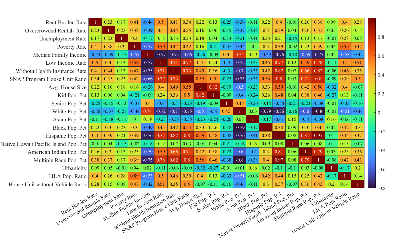
Figure 1 presents a heatmap of the correlation matrix for the 21 variables and it reveals some key relationships.

Socioeconomic status.

There are strong positive correlations among lack of health insurance, low income, and reliance on SNAP programs. In contrast, higher median family incomes are associated with greater financial stability and negatively correlated with the above indicators. Additionally, rental burden, overcrowding, and poverty rates are moderately linked, suggesting interconnected housing and economic challenges. Meanwhile, unemployment is moderately tied to poverty but has weaker connections to other socioeconomic factors.

Household composition.

Average house size tends to increase with kid population ratio, as one would expect. Urbanicity is moderately associated with both house size and kid population ratio, but its relationships with other variables are relatively weak.

Demographic ethnicity.

Minority groups such as Hispanic, Multi-race, and American Indian populations are more likely to experience socioeconomic stress, as evidenced by positive correlations with low income, SNAP program usage, and lack of health insurance. Conversely, the White population tends to show negative correlations with these indicators. The Native Hawaiian Pacific Islander population has weak correlations due to its small size and limited impact on census tract composition.

Accessibility.

Households without vehicles and LILA populations tend to experience higher rates of socioeconomic difficulties, including low income and poverty, which is consistent with expectations.

Solving the 21×21 covariance matrix yielded 21 eigenvectors and corresponding eigenvalues. The eigenvalues determine the variance explained by each component. Applying the Kaiser criterion, components with eigenvalues greater or equal to 1 were retained as PCs. Figure 2 presents the scree plot, labeling variance on the left and eigenvalues on the right. The plot indicates that only five components have eigenvalues greater than one. The PC1 has an eigenvalue of 8.68, explaining 41.33% of the information from the 21 variables, while PC5 has an eigenvalue of 1.07, accounting for 5.09% of the variance. In total, the top five PCs explain 71.15% of the variance.

Table 1 presents the coefficients of each variable in the top five PCs after applying Varimax rotation. To identify primary contributors, a loading threshold of 2/3 was applied. Variables meeting or exceeding this threshold are highlighted in the table. PC1’s key drivers include socioeconomic indicators such as “Without health insurance population rate,” “Low-income rate,” “SNAP program house unit ratio,” and “Median income,” as well as racial/ethnic variables like “American Indian population percentage,” “Hispanic population percentage,” and “Multiple race population percentage.” These variables exhibit strong positive and negative correlations, as evident in the correlation heatmap. Notably, higher median incomes enhance food security and reduce risk, whereas areas with high percentages of low-income individuals, SNAP program households, and uninsured populations are more vulnerable to food insecurity. This relationship is reflected in the negative weights assigned to these variables. Additionally, the negative weights for the census tracts with higher ratios of American Indian, Hispanic, and Multiple race populations suggest that these areas face greater food insecurity challenges compared to those with higher proportions of White and Asian populations.

Table 1. Weight values for each variable of principal components after Varimax rotation
Variable of Census Tract	PC1	PC2	PC3	PC4	PC5
Rent Burden Rate	-0.3860	0.0234	-0.0688	-0.4421	-0.0227
Overcrowded Rentals Rate	-0.3873	0.0218	0.0640	-0.4078	0.0175
Unemployment Rate	0.0541	-0.2359	0.2504	-0.6897	-0.0951
Poverty Rate	-0.3965	0.2418	-0.1648	-0.7355	-0.0560
Median Family Income	0.7735	-0.0086	0.2598	0.3661	0.0288
Low Income Rate	-0.7998	-0.0725	-0.1983	-0.3518	0.0227
Without Health Insurance Rate	-0.8146	-0.1965	-0.0589	-0.2493	0.0699
SNAP Program House Unit Ratio	-0.7848	-0.3831	0.0154	-0.2233	-0.0860
Avg. House Size	-0.3195	-0.7913	-0.0050	-0.1796	0.2872
Kid Population Pct	-0.2650	-0.8676	0.0316	0.1486	0.1957
Senior Population Pct	0.2311	0.1159	0.6367	0.2811	0.0868
White Population Pct	0.6484	0.4492	0.3388	0.3296	0.2748
Asian Population Pct	0.4883	0.0561	-0.6422	-0.0332	-0.2972
Black Population Pct	-0.3317	-0.4409	-0.1350	-0.3831	-0.3284
Hispanic Population Pct	-0.8757	-0.3184	-0.0466	-0.1843	0.0761
Native Hawaii Pacific Island Population Pct	-0.1254	0.0535	-0.6845	0.1866	0.2578
American Indian Population Pct	-0.8182	-0.2472	0.0601	0.0288	-0.0584
Multiple Race Population Pct	-0.8844	-0.3121	-0.0747	-0.1535	0.0179
Urbanicity	0.0090	0.1859	0.0291	0.0634	-0.7896
Low Income Low Access Population Ratio	-0.2826	-0.1401	-0.2845	-0.6875	0.2338
House Unit without Vehicle Ratio	-0.5735	0.2370	0.0210	-0.1595	-0.4691

The subsequent components reveal additional insights into food insecurity. PC2, accounting for 10.8% of the total variance, suggests that larger households with more children are more vulnerable to food insecurity, likely due to increased food requirements and family burdens. PC3 is characterized by a strong presence of “Native Hawaii Pacific Island Population Ratio”, with “Asian population ratio” and “Senior population ratio” (slightly lower than threshold) also aligning with this component. Notably, these variables exhibit weak correlations with other variables, indicating distinct and non-redundant information. In contrast, PC4 reveals a strong negative relationship between food security risk and socioeconomic indicators, including unemployment rate, poverty rate, and LILA population ratio, aligning with expectations. Finally, PC5 is primarily defined by accessibility factors, particularly “Urbanicity” and “House unit without vehicle”. These variables display weak correlations with other variables, forming a distinct cluster in this component.

To construct food insecurity risk index, the five principal components value of each census tract are re-casted through a weighted linear summation, as formulated in Eq. 2:

\[Comp\_value\left(i,\ n\right)=\sum_{k=1}^{21}{X\left(i,k\right)W_1\left(k,n\right)}\tag{2}\]

Here i, n and k are indices of census tracts, PCs, and independent variables, respectively. Comp_value(i,n) denotes the value of the n^th PC for i^th census tract, X(i,k) is the normalized k^th variable value for i^th census tract, and W₁(k,n) corresponds to the weight coefficient of k^th variable in n^th PC listed in table 1.

A composite food insecurity risk score is computed for each census tract using Eq. 3:

\[Risk\_Score\left(i\right)=\sum_{k=1}^{5}{Comp\_Value\left(i,k\right)W_2\left(k\right)}\tag{3}\]

Here are W₂(k) the weight coefficients assigned according to variance explained by each of the five PCs. The resulting risk scores are then normalized to z-scores based on score standard deviations. Figure 3 illustrates the distribution of these z-scores across 217 census tracts in Travis County, excluding one tract designated as an airport area.

A geospatial map of food security risk is created in QGIS as shown in Figure 4, categorizing risk scores into 7 levels based on standard deviations of their risk values with darker blue areas indicating higher risk census tracts. The yellow dots on the map represent CTFB service locations.

DISCUSSION.

This study employed PCA and GIS mapping techniques to aggregate household food insecurity data at a census tract level. The results revealed a concentration of high-risk areas in central east Travis County (downtown Austin), aligning with CTFB service location distributions. Geographic analysis showed that the east Travis County area has a higher minority population and poverty rates which correspond to increased food insecurity risk, whereas west Travis County has more affluent communities which exhibit lower risk. Rural areas in northwestern Travis County displayed moderate risk, and CTFB has some food service locations put in place. This research corroborates previous social studies [9] in Austin, highlighting the disproportionate socioeconomic challenges faced by east Austin communities relative to those in west Austin. CTFB currently relies on volunteer-led surveys to determine optimal food service locations, a resource-intensive process, particularly in rural areas. Our PCA-based approach streamlines this process, allowing for data-driven decision-making and targeted resource deployment to areas with greatest need.

ACKNOWLEDGMENTS.

I would like to thank the staff of the Central Texas Food Bank for their support with my research.

REFERENCES.

1. A. Rhone, R. Williams and C. Dicken, Low-income and low food store-access census tracts, 2015-19. USDA Economic Research Service, Economic Information Bulletin, No. 236 (2022)
2. M. P. Rabbitt, L. J. Haels, M. P. Burke and A. Coleman-Jensen, Household food security in the United States in 2022, USDA Report (2023).
3. M. Hake, E. Engelhard and A. Dewey, Map the meal gap 2023 https://www.feedingamerica.org/sites/default/files/2023-05/Map the Meal Gap 2023.pdf
4. K.M. Janda, N. Ranjit, D. Salvo, D. Hoelscher, A Nielsen, J. Casnovsky and A. Berg, Examining Geographic food access, food insecurity, and urbanicity among diverse, low-income participants in Austin, Texas, Int. J. Environmental Research and Public Health, 19(9), 5108 (2022).
5. M.S. Livings, W.B. Bruin, J.P. Wilson, M. Babboni and K.D. Haye, Food insecurity is under-reported in surveys that ask about the past year, American J. of Preventive Medicine, 65(4), 657-666 (2023).
6. T. Burgoine, S. Alvanides and A.A. Lake, Creating ‘obesogenic realities’; do our methodological choices make a difference when measuring the food environment? Int. J. Health Geography, 12, 33 (2013,).
7. United States Census Bureau American Community Survey (ACS) dataset. https://www.census.gov/programs-surveys/acs
8. H. F. Kaiser, & J. Rice, Little jiffy, mark IV, Educational and Psychological Measurement, 34(1), 111-117 (1974).
9. M.K. Lasode, T.E. Chow, R.R. Hagelman, R.D. Blanchard, O.O. Lasode, A.E. Iyanda, The impact of homelessness in social vulnerability assessment: a case study of Austin, Texas. Social and Economic Geography, 6(1), 1-12 (2021).

---

---

Posted by buchanle on Wednesday, July 16, 2025 in May 2025.

Tags: Food Insecurity, Geographic Information Systems (GIS), Principal Component Analysis (PCA), Risk Assessment