Tracking river movement and delta formation by analyzing sediment from the Brahmaputra river
ABSTRACT
Currently, about 40% of the world’s population lives near the coast. These regions face many challenges including sea level rise, increased human development, and natural disasters. In order to better understand and predict both natural and artificially caused developments, both current and future, it is important to understand how these landscapes develop and change over time. Sitting on three active tectonic plates, Bangladesh has a geologically complex coastal system with the world’s largest river delta. The Brahmaputra, Meghna, and Ganges rivers erode and distribute approximately 1.0´109 tons of sediment from the Himalayas to build this delta every year. Past research has shown that strontium can be used as a trace element to accurately identify the specific origin of Himalayan derived sediments. Using this method, researchers were able to find Pleistocene aged Brahmaputra derived sediments that could not have been deposited if the river were where it is today. This research focuses on the down-stream fining of these Brahmaputra derived sediments in order to understand the causes of this river movement. Unexpected results showed that the area did not follow typical fining patterns. These results were compared to those from Holocene Brahmaputra sediments to analyze the differences between these patterns and learn more about the river’s behavior.
INTRODUCTION.
Approximately 40% of the world’s population, about 2.4 billion people, currently lives within 100 kilometers of a coast [1]. Coastal systems are faced with issues resulting from sea-level rise, increasing human impact on earth processes, and events such as natural disasters like typhoons and tsunamis [1]. With the vast number of people living near the coast, it is important to understand how coastal systems work and develop over time in order to better predict future coastal developments and be prepared for changes in the environment.
With three major rivers, the Ganges, Brahmaputra, and Meghna, Bangladesh has a geologically complex and interconnected landscape that is home to the world’s largest delta. This coastal landscape sits on top of several active tectonic plates, including the Indian and Eurasian, that create key formations including the Shillong Plateau, the Tripura fold belt, and the Himalayan collision zone. As the rivers flow through these regions, sediment is eroded and carried downstream where the deposits contribute to the developing landscape. Through past research the Ganges-Brahmaputra-Meghna Delta (GBMD) has been categorized as a composite system, a type of delta that is composed of different systems working together [2]. This previous work categorized regions as either in a state of construction, maintenance, or decline where sediment deposition rates exceeded, met, or were below rates of sea-level rise respectively. This information can be used to evaluate flood risk in these areas and help local populations be better aware and prepared.
Previous research has shown strontium to be effective as a trace element for Himalayan derived sediments in Bangladesh [3], [4]. By measuring strontium concentration, the river from which these sediments were deposited can be identified. This method was used to identify the source river for sediment in several areas of the lower delta. Due to a significant percent of Brahmaputra derived sediments, [3] were able to find that the Brahmaputra river has migrated west across the delta throughout the Pleistocene Epoch.
Sediment grain size is another effective way of identifying deposit origins [5]. As a result of differences in mineral composition and weathering, sediments vary over a wide range of sizes and densities. As the river deposits them, the larger, denser, sands are deposited first, closer to the site of erosion, while the finer particles such as clay and silt are suspended in the water column for a longer period of time and are deposited farther downstream. The concept of deposits varying in size down the delta due to varying densities is known as downstream fining and can be used to help determine where the site of erosion is for a certain area.
This paper looks to find the cause for migration of the Brahmaputra River to central Bangladesh by comparing the downstream fining of Pleistocene sediments and Holocene sediments. It has been hypothesized that the uplift of the Shillong Massif during the Pleistocene forced the Brahmaputra river west. This hypothesis will be tested by comparing the average grain size of Holocene and Pleistocene aged sediments at varying depths of cores spanning down the delta. Many cores (boreholes) contain both Pleistocene and Holocene aged sediments because more recent, Holocene sediments were deposited after and therefore on top of the Pleistocene sediments. If the Pleistocene sediments were much coarser than it is likely migration was caused by uplift of the Plateau. However, if the sediments are less coarse than those of the Holocene, it is more likely that they came from the more distant Himalayas.
MATERIALS AND METHODS.
Boreholes from the Pleistocene Brahmaputra river bed from the T2, T3, and G- transects as well as cores 2,3, and 5 were collected for previous work by Goodbred et al. using the hand-drilled reverse circulation method (Fig. 1c). Core 4 was the only one collected using a hollow-stem auger with a split spoon sampler [3]. Samples from transects T-2, T-3, and G, (Fig. 1a), were taken at 1.5-m intervals throughout the boreholes. This research uses data from 26 cores and 393 samples from the Pleistocene and 52 cores and 971 samples from the Holocene. A Malvern Mastersizer 2000 Particle Size Analyzer was used to determine the size of the sediment grains in each sample.
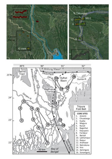
Figure 1a. Satellite Image of the Bengal Basin with upper (transect T-2 and T-3), lower delta, and G cores from the Pleistocene outlined in black and the Brahmaputra river outlined in blue. 1b) Satellite Image of Bengal Basin with upper (transect T-2, A, and SH1 and SH2), lower delta (X), and G cores from the Holocene outlined in black and the Brahmaputra river outlined in blue. 1c) Map of cores used in (Goodbred et al., 2014) to verify efficacy of strontium as a trace element. This research used data from cores 5, 6, 7, 8, and 9, which were found to have been deposited by the Brahmaputra River.
Sediment samples were mixed with water and passed through a small window in the Mastersizer. A 1,000 mL beaker was filled with deionized water and put under the machine’s pump which was then turned on and off until all bubbles had been removed from the water, because air bubbles diffract the laser light, creating excess noise in the data. The instrument then measured background laser absorption of the plain water and beaker. The sediment samples were prepared by scooping ˂ 1 g into a 1,000 µm sieve over a pan. Deionized water was used to move the particles through the sieve. This slurry was then added to the 1,000 mL beaker and subjected to an ultrasound for 20 seconds, which uses high-frequency sound to disaggregate any clustered sediment particles. Laser light passed through the windows where it was diffracted as it hit the sediment particles. The angle of diffraction caused by the sediment grains was then used by the Mastersizer program software to calculate the mean grain size and size distribution of the particles.
The resulting size distribution of sediment particles can be used to understand how close the deposit site may be from the rock source and what the transport energy of the water flow may have been when it was deposited. Such information can be used to understand how sediment was delivered to the delta to build the landscape. These patterns were analyzed by finding the average grain size at each depth across the transects and calculating the percentage composition of each sediment type and the fraction of fine (125-250 µm), medium (250-500 µm), and coarse sands (500-1,000 µm). Fine, medium, ad coarse sand percentages were calculated by normalizing the data after excluding clay, silt, and very fine sand. Based on our hypothesis, if the sediment from the Pleistocene is much coarser than that in the Holocene, then it may likely have come from the uplifted Shillong Massif. However, if the sediment from the Pleistocene is finer than that in the Holocene, then it likely came from the Himalayas.
Sunil Singh and Christian France-Lanord studied strontium in marine settings from the Miocene and Pleistocene and used the isotopes to identify changes in the rate of Himalayan erosion over time [4]. They found that strontium isotopes could be used to find sediment provenance from the Himalayas [5]. Goodbred et al. [2] later verified that strontium concentration, which is easier and less expensive than Sr isotopes to measure, was also a reasonably accurate trace element for identifying the origin of sediment deposits in the GBMD. Using X-ray fluorescence (XRF), they found Pleistocene deposits from the central-low area of the basin (cores 5,6,7,8, and 9) (fig. 1c) to contain a large amount of Brahmaputra derived sediments. With the knowledge that these sediments, along with T2, T3, and G transect core samples, were deposited by the Brahmaputra, comparisons can be made between Holocene and Pleistocene sediments with the same provenance to find differences in downstream fining patterns between the epochs.
RESULTS.
Pleistocene sample depths measured in respect to the Pleistocene surface. Holocene sample depths were measured in respect to the Holocene surface. The average grain size of Pleistocene cores tended to be finer towards the surface before gradually increasing with depth (fig. 2a). Figure 2a shows an average trend of 350-450 µm with finer sediments closer to the surface. Excluding the Magura core, all cores show a similar pattern of having finer sediments towards the surface and gradually become coarser as they get deeper. The T2 and T3 cores show similar patterns. They both have a slight decrease in average grain size around 35 m in depth below the Holocene-Pleistocene boundary and then display a momentary increase at 40 m depth. On average, T3 remains slightly coarser, ranging from 380 µm-480 µm, than T2, ranging from 340 µm-400 µm, across the depths. Narail begins coarser than the other cores but quickly becomes finer around 10 m depth. The G transect and Kustia/Chuadanga cores follow similar patterns to the T transect cores. Unlike the other cores, Magura, does not have the cap of finer sediments, but remains fairly consistent towards the surface. Around 40 m depth, the average grain size decreases before gradually increasing until 60 m depth where it begins to fluctuate more as the core gets deeper.
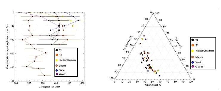
Figure 2. Average grain size of Pleistocene sediments at varying depths in respect to the Pleistocene surface for 6 core averages (left). Percentage of fine, medium, and coarse sand averaged by depth for each group of Pleistocene cores (right). Error bars represent the standard deviation of the cores at each depth.
In figure 2b, the cores differ in coarse and fine sand percentages more than in medium sand percentages. The Magura core displays a higher percentage of fine sand than coarse sand and is similar to the other cores for medium sand percentage. This plot supports results of the depth and grain size plot because it excludes silt and clay-sized sediments from the percentages and only shows sand. These results demonstrate that the cores are more or less coarse because of the sand make-up and independent of the amount of silt or clay.
In figure 3a, the average grain size of the Holocene sediments becomes coarser with depth on a linear pattern. T-2 and A, ranging between 300 and 500 µm, are similar throughout the various depths and are on average coarser than the other two cores. Ranging between 250 and 400 µm, the X core averages are finer than those of T-2 and A, but coarser than the G transect cores. The X cores show a slight decrease in average grain size between 20 and 35 m in depth. The G cores average between 150 and 350 µm and are finer than both the X, T-2, and A transect cores.
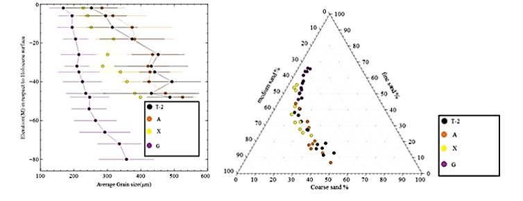
Figure 3a. Average grain size of 4 Holocene dated cores at various depths (left). Ternary plot of fine, medium, and coarse sand percentages within 4 Holocene cores (right). Error bars represent the standard deviation of the cores at each depth.
In figure 3b, cores vary the most in fine sand, then coarse sand, and least in medium sand percentage composition. The majority of T-2 transect core sands come from coarse and/or medium sands and are fairly consistent in composition between the depths. On average, the percentage of medium sand in A transect cores remain between 55 % and 65%, however, coarse and fine sand percentages are more variable. The majority of X- transect sands were either medium or fine with coarse percentages consistently averaging under 30%. G transect cores are highest in fine sand, ranging between 45% and 65% and lowest in coarse sand averaging under 10%. This supports the findings from average grain size by only including coarse, medium, and fine sand. By excluding silts, it can be seen how much the sands vary in coarseness between each core rather than get an average. Specific differences and similarities can be seen when comparing the results of the two scatter plots (fig. 2a and 3a). In both figures 2a and 3a, transects T-2 and T-3 (transect A for the Holocene) were similar in mean grain size throughout the depths. However, this mean grain size is different between the Pleistocene and Holocene sediment packages. T-2 and T-3 sediments from the Pleistocene ranged between 350 and 450 µm while geographically comparable sediments from the Holocene followed a more linear progression of mean grain size with depth and therefore did not stay within a defined range. They did, however, prove to be coarser than Pleistocene sediments.
When comparing the two ternary points (Fig. 2b and 3b), it can be seen that in both the Pleistocene and Holocene, coarse and fine sand fluctuate more than medium sand between each sample. However, medium sand changes more during the Holocene than it does in the Pleistocene. In both the Pleistocene and Holocene, the T-2 transect cores average between 30% and 50% coarse sand, 50% and 60% medium sand, and 10% and 20% fine sand. The T-3 and A transects vary more between the epochs. While the T-3 transect is similar to the T-2 transect in the Pleistocene, the A transect varies more in coarse and fine sand.
The average grain size of the G cores from the Holocene are not similar to G core sediment grain sizes from the Pleistocene. Sediments from the Holocene follow a linear progression of increasing grain size with depth and on average are < 350 µm. Sediments from the Pleistocene, however, follow an exponential-like pattern and range between 350 and 430 µm. This linear versus exponential pattern is a trend throughout both epochs. Holocene sediments from the X transect are more similar in grain size to Pleistocene sediments from the G transect. Holocene sediments from the G transect would be more similar to Pleistocene sediments from the Magura core in both average grain size and trend.
DISCUSSION.
The results from grain size analysis and percent make-up during the Pleistocene do not follow typical trends of down-stream fining. Typically, sediments fine down delta due to fluvial depositional processes. However, that was not the case here. Due to these results, the sediment origin cannot be indefinitely determined. It is possible that different areas of the Pleistocene delta were derived from different sources rather than one location.
Prior research found that differing grain sizes dominated areas with certain conditions [6]. Coarse sand tends to dominate areas with “high-energy fluvial processes”, fine sand tends to dominate areas with active tectonics including subsidence, and mixed sands tend to dominate areas subject to sea level change [6]. In past studies, scientists identified areas throughout the delta as either being in phases of construction, maintenance, or decline [1]. Construction occurs when the rate of sediment deposition is greater than the rate of subsidence; maintenance occurs when the rate of sediment deposition is equal to the rate of subsidence, and decline occurs when the rate of sediment deposition is less than the rate of subsidence [1]. By extrapolating these results to the Pleistocene, areas of high subsidence could account for areas high in fine sand while high energy systems could account for coarser areas. Results in McLaren and Bowels [7] supports the theory of coarse sediments being preferentially deposited in high energy distribution systems. It is possible that the upper delta was steeper during the Pleistocene causing an increase in river energy. This increase would allow coarser sediments to be suspended for a longer period of time and deposited further down the delta. Future studies will look more in depth at gravel content in order to get a more complete picture of sediment make-up and better identify sediment origins.
Philip Allen highlights the need to take an interdisciplinary approach when looking at Earth surface processes [8]. Atmospheric and oceanographic factors can be just as important as geologic factors in systems such as deltas [8]. It is possible that factors not recorded or recorded differently were highly influential in delta construction during the Pleistocene.
This research provides an account of how this region of Bangladesh could have been constructed during the Pleistocene. It also provides details of river movement throughout the history of the landscape that can be used to help understand river movement and construction now.
ACKNOWLEDGMENTS.
I would like to thank Dr. Steven Goodbred for allowing me to conduct research in his lab and guiding me throughout the project. I would also like to thank my mentor, Jessica Raff, for assisting me every step of the way and Dr. Nathan Haag, my advisor, for being a constant support. Thank you to the School for Science and Math at Vanderbilt for giving me this amazing opportunity.
REFERENCES.
- UN.org, “Factsheet:People and Oceans”, 2107. [online]. Available: https://www.un.org/sustainabledevelopment/wp-content/uploads/2017/05/Ocean-fact-sheet-package.pdf. [Accessed: 17-Aug-2019].
- C. A. Wilson, S. L. Goodbred, Construction and Maintenance of the Ganges-Brahmaputra-Meghna Delta: Linking Process, Morphology, and Stratigraphy. Ann. Rev. Mar. Sci. 7, 67-88 (2014).
- S. L. Goodbred et al, Piecing together the Ganges-Brahmaputra-Meghna river delta: Use of sediment provenance to reconstruct the history and interaction of multiple fluvial systems during Holocene delta evolution. Bull. Geol. Soc. Am. 126, 1495-1510 (2014)
- S. K. S. Ã et al, Tracing the distribution of erosion in the Brahmaputra watershed from isotopic compositions of stream sediments. Earth Planet. Sci. Lett. 202, 645-662 (2002)
- L. A. Derry, C. France-Lanord, Neogene Himalayan weathering history and river87Sr86Sr: impact on the marine Sr record. Earth Planet. Sci. Lett. 142, 59-74 (1996)
- S. L. Goodbred, S. A. Kuehl, M. S. Steckler, M. H. Sarker, Controls on facies distribution and stratigraphic preservation in the Ganges-Brahmaputra delta sequence. Sediment. Geol. 155, 301-316 (2003)
- P. McLaren, D. Bowles, The effects of sediment transport on grain-size distributions. J. Sediment. Petrol. 55, 457-470 (1985)
- P. A. Allen, From landscapes into geological history. Nature. 451, 274-276 (2008)
Posted by John Lee on Wednesday, December 23, 2020 in May 2020.
Tags: Delta Formation, river migration, sediment distribution